Published by:
Aardsma Research & Publishing
301 East Jefferson Street
Loda, Illinois 60948

biblicalchronologist.org
agingcauseandcure.com

Printed in the United States of America

Library of Congress Control Number: 2023911448

ISBN 978-1-7372151-3-4

Contents

List of Tables	11
List of Figures	13
Dedication	17
Acknowledgments	19
Preface	21
1  Beginnings	27
1.1  Cleaning the Slate	27
1.1.1  "Aging"	27
1.1.2  Impact of Modern Medicine on Maximum Life Span	28
1.1.3  "Special" Groups and Individuals	29
1.1.4  "Normal" Life Span	30
1.2  A New Hypothesis	30
1.2.1  "Old Age"	31
1.2.2  The Number One Health Problem	32
1.3  The Difficulty of the Research Problem	33
1.4  Conclusion	34
2  Understanding the Essence of Aging	35
2.1  Getting the Wrong Idea About Aging	35
2.2  Two Questions	36
2.3  The Essence of Aging	37
2.3.1  Time's Role	37
2.3.2  The Congenital Diseases of Aging	38
2.4  Deriving the General Theory of Aging for Biological Organisms	39
2.4.1  Survival Curves	39
2.4.2  The Gompertz Function	42
2.4.3  A Thought Experiment	44
2.5  Conclusion	48
3  Understanding the Etiology of Aging	49
3.1  A General Theory of Aging	50
3.1.1  Longevity and Natural Selection	51
3.1.2  Impediments to Increasing Longevity	53
3.2  Conclusion	54
4  Modeling Survival Curves in Light of the General Theory of Aging	57
4.1  Data Analysis Method	57
4.2  The Model	58
4.3  Beyond Gompertz	61
4.4  Weighting the Fit	63
4.5  Performing the Least-Squares Fit	64
4.5.1  Post-fit Scaling of Uncertainties	65
4.6  Separation of Signal from Noise	67
4.7  Conclusion	69
5  The Biblical History of Human Aging	71
5.1  Life Spans	71
5.2  Birthdates	74
5.3  Life Expectancy	76
5.4  Conclusion	78
6  The Biblical Life Expectancy Graph	79
6.1  A Powerful Instrument	80
6.1.1  Supernatural	80
6.1.2  Vapor Canopy	82
6.1.3  Evolution	83
6.1.4  General Theory of Aging	84
6.2  Conclusion	87
7  The Central Hypothesis	89
7.1  Deficiency Diseases	89
7.1.1  The Example of Vitamin C	90
7.2  Working Hypothesis	92
7.2.1  Complex of Symptoms	93
7.2.2  Particular Symptoms	93
7.2.3  Apparent Contrast	94
7.2.4  Variable Time of Onset	94
7.2.5  Why Life Spans Changed	95
7.3  Conclusion	95
8  Properties of Vitamin X	97
8.1  The Eber–Peleg Drop	97
8.2  Biological Half-life	99
8.3  Biological Half-life of Vitamin X	99
8.4  Environmental Half-life of Vitamin X	101
8.5  Conclusion	102
9  The Environmental Abundance of Vitamin X	103
9.1  The Environmental Abundance Graph	103
9.1.1  The Post-Peleg Decline	104
9.1.2  The Moses Drop	104
9.2  Conclusion	106
10  The Natural Synthesis and Distribution of Vitamin X	109
10.1  How Was Vitamin X Distributed by Nature?	109
10.2  How Was Vitamin X Synthesized by Nature?	111
10.3  How Did Vitamin X Enter the Human Diet?	112
10.4  The MSA Example	112
10.5  Conclusion	113
11  What the Flood Broke	115
11.1  The Nature of the Flood	115
11.2  The Nature of Sea Floors	116
11.3  The Source of the Precursor	117
11.4  Conclusion	117
12  Vitamin X Candidates	119
12.1  A Phosphorus Trace Gas	120
12.1.1  Methylated Phosphorus Gases	123
12.2  Conclusion	129
13  Choosing Vitamin X	131
13.1  The Data	132
13.2  Is it Real?	134
13.3  Discussion	136
13.4  Check	136
13.4.1  Correction 1: Megadose MePiA is Toxic	138
13.4.2  Correction 2: MePA is Efficacious With Mice	140
13.4.3  Correction 3: Megadose MePA is Toxic	140
13.4.4  Correction 4: Vitamin X is a Vitamin Duo	142
13.5  The Theory of Modern Human Aging	142
13.6  Conclusion	143
14  Early Experiences With MePA	145
14.1  Assessing Benefit Versus Risk	145
14.2  MePA Versus "Old Age"	146
14.2.1  CIDP	147
14.2.2  Skin	149
14.2.3  Sleep	150
14.2.4  Headache/Migraine	151
14.2.5  Upper Respiratory Infections	152
14.2.6  Helen Corroborates My Early Experience	152
14.2.7  Rate of Healing	153
14.2.8  Weight	154
14.2.9  Arthritis	155
14.2.10  More Observations from Helen	156
14.3  Conclusion	158
15  Vitamin MePA	159
15.1  MePA–a New Vitamin?	159
15.1.1  Anti-aging Vitamins Predicted	159
15.1.2  MePA Behaves Similar to Other Vitamins	160
15.1.3  MePA is Vitamin-Like, Not Drug-Like	163
15.1.4  MePA Satisfies the Criteria for a Vitamin	164
15.2  The Cure for MePA Deficiency Disease	166
15.2.1  Recommended Daily Intake	167
15.3  Conclusion	167
16  Inadvertent Experience With MePiA	169
16.1  The Difficulty of Crediting Symptoms to MePiA	169
16.2  An Inadvertent Experiment	170
16.3  Conclusion	172
17  Vitamin MePiA	175
17.1  MePiA is Another New Vitamin	175
17.2  The Cure for MePiA Deficiency Disease	176
17.2.1  Recommended Daily Intake of MePiA	176
17.2.2  Overdosing	177
17.2.3  Present Recommendation	178
17.3  Conclusion	178
18  Explaining Modern Human Life Spans	181
18.1  Defining the Problem	181
18.2  The Modern Actuarial Dataset	182
18.3  Review	183
18.4  Method	184
18.4.1  Step 1: Model a Single Aging Disease	184
18.4.2  Step 2: Fit the First-Approximation Model to the Modern Male Life Span Dataset	185
18.4.3  Step 3: Change the Model to Describe Saturation of MePiA Deficiency Disease	193
18.4.4  Step 4: Upgrade the Model to Include MePA Deficiency Disease	197
18.5  Discussion	198
18.6  Conclusion	201
19  Explaining Ancient Historical Human Life Spans	203
19.1  The Model	204
19.1.1  Details	204
19.2  Results	210
19.2.1  Environmental Free Parameters	210
19.2.2  Physiological Free Parameter	212
19.3  Conclusion	212
20  Potential Longevity Today	215
20.1  Method	216
20.1.1  Life Expectancy	216
20.1.2  Computer Program	217
20.2  Results	223
20.3  Discussion	226
20.4  Conclusion	229
21  How to Maximize Your Health and Longevity Starting Now	231
21.1  Rule 1	232
21.2  Rule 2	234
21.3  Conclusion	235
Appendices	237
A  PODfit10.F95	239
B  MeP_20230509.F95	267
C  ACAC3_actuarial_table.F95	281
Index	289

List of Tables

5.1  Selected biblical life span data.	73
5.2  Birthdates of selected biblical males.	75
5.3  Point estimates of life expectancies from Adam to Moses.	77
18.1  Numbers of deaths in 2016 resulting from MePiA and MePA deficiency diseases.	198
20.1  Life expectancy increase factor versus age of starting supplementation with the anti-aging vitamins for ages 1 to 113 years.	223

List of Figures

2.1  Survival curve data for fruit flies.	40
2.2  Survival curve data for modern U.S. males.	41
2.3  Gompertz function fit to survival curve data for fruit flies.	43
2.4  Gompertz function fit to survival curve data for modern U.S. males.	44
2.5  Survival curve for men due to starvation beginning at age 25 years.	46
3.1  Bristlecone pine tree.	55
4.1  Survival curve data for modern U.S. males.	58
4.2  Survival curve data for modern U.S. males with least-squares fit of the Aardsma model.	65
4.3  Survival curve data for modern U.S. males with estimated survival curves in the absence of aging and in the absence of random deaths.	68
5.1  Biblical data showing life expectancy at birth for selected males.	78
6.1  Measured temperature versus time for a bowl of hot water.	81
6.2  Survival curve data for modern and ancient males with least-squares fit curves of the Aardsma model.	85
7.1  Structure of the vitamin C molecule.	91
8.1  The Eber–Peleg Drop.	98
9.1  The Eber–Peleg Drop, Post-Peleg Decline, and the Moses Drop.	105
9.2  Pre-Flood, Spike, Decline, and Modern time periods.	107
12.1  Oceanic phosphate surface distribution.	121
12.2  Oceanic nitrate surface distribution.	121
12.3  The MeP, MePiA, and MePA molecules.	126
13.1  Survival curve datasets for the MePA-vs-MePiA-treated ICR female weanling mice experiment.	133
13.2  Survival curve datasets for the MePA-vs-MePiA-treated ICR female weanling mice experiment with three additional batches of the same type of mice.	135
13.3  Survival curve datasets for the second ICR female weanling mice experiment.	137
13.4  Survival curve datasets for the first and second ICR female weanling mice experiments at 0.1 g MePiA/L.	139
13.5  Survival curve datasets for ICR female weanling mice showing life lengthening due to MePA and chronic toxicity of megadose MePA.	141
15.1  Geriatric features in a niacin-deficient, 6-month-old pig.	160
18.1  Survival curve data with least-squares fits for U.S. males and females for the year 2016.	183
18.2  2016 actuarial life table probability-of-death-per-year data for U.S. males.	187
18.3  2016 actuarial life table data for U.S. males with the probability-of-death-per-year axis expanded by a factor of 100.	189
18.4  2016 actuarial life table data for U.S. males with the probability-of-death-per-year axis expanded by a factor of 1000.	190
18.5  2016 actuarial life table data for U.S. males with weighted least-squares fit of the Equation 18.4 model to selected data points.	191
18.6  2016 actuarial life table data for U.S. males with weighted least-squares fit of the Equation 18.8 model to selected data points.	197
18.7  Least-squares fit of the final model to the 2016 actuarial life table data for U.S. males.	199
18.8  Least-squares fit of the final model to the 2016 actuarial life table data for U.S. females.	200
19.1  Results of the biblical life span data model.	205
20.1  Life expectancy for modern U.S. males and females not taking the anti-aging vitamins.	217
20.2  Survival curves for U.S. females supplementing with the anti-aging vitamins and not supplementing with the anti-aging vitamins.	227
21.1  Life expectancy increase factor for U.S. males and females starting to take the anti-aging vitamins.	231
21.2  Life expectancies for U.S. males and females starting to take the anti-aging vitamins and not starting to take the anti-aging vitamins.	233

The following dedication, from the first edition, expresses sentiments which only grow deeper with each new edition and each passing year.

To Helen,

How many times have we looked at one another these past seventeen years and recited those words from David Mamet's film, The Winslow Boy, "Are we crazy, you and I?"

Thank you for choosing to walk this difficult road with me. You have been a friend encouraging me to press on, a secretary running the business, a comrade covering my back, a nurse watching by my bedside, a business partner financing her research scientist, a teammate setting me up for the shot, … and all the while a poverty-line housewife looking after her children and her man. How can I not admire you?

Well, now we have the answer. It seems we were not crazy after all. And I am so looking forward to growing young with you.

Gerald
July, 2017

To this the following heartfelt sentiment is added this edition.

And to

Matthew, Esther, Ger, Ellie, Adaline, Mimi, and William,

whom my soul loves.

I wish to express my sincere appreciation to: 1) Matthew Aardsma for his contributions to the second edition of this book from his expertise in animal nutrition, some of which have been ported over into this third edition, 2) Tom Godfrey for general proofreading and editing assistance as well as compilation of the index, and 3) Steve and Jennifer Hall for proofreading, discussions of the present content, graphic design and artwork, and seeing this volume through the printing process.

So at last Faramir and Éowyn and Meriadoc were laid in beds in the Houses of Healing; and there they were tended well. For though all lore was in these latter days fallen from its fullness of old, the leechcraft of Gondor was still wise, and skilled in the healing of wound and of hurt, and all such sickness as east of the Sea mortal men were subject to. Save old age only. For that they had found no cure…^[1]

I am a research scientist. I have spent most of my life researching at the interface of science and the Bible. My science specialty is physical dating methods such as radiocarbon. My earliest full-time Bible/science research effort centered around the question of why nobody had ever been able to pin a functional historical date on Noah's Flood. This led, eventually, to the discovery that exactly 1000 years had been accidentally dropped from traditional biblical chronology due to an inadvertent copy error in a number found in 1 Kings 6:1.^[2]

This rapidly led to answers to other Bible/science questions I had not even set out to investigate. For most of the final decade of the twentieth century, I was immersed in research connected to the Exodus of Israel from Egypt, the ensuing Conquest of Canaan, and the much earlier-in-time Flood of Noah. I found that the Exodus was a real historical event, and that the biblical description of it was simply historical.^[3] Many scholars were saying the opposite, but that was because they had their biblical chronology wrong by 1000 years. You cannot find an object if you spend all your time looking for it a thousand miles from where it is located, and you cannot find a historical event if you spend all your time looking for it one thousand years from when it happened.

Also severely in conflict with mainstream scholarship, I found that the Flood, too, was a real historical event, and that the biblical record of it, too, was simply historical. Mainstream scholarship has held for some decades that the Flood is mere legend.

The lengths of reign of the earliest kings [of the Sumerian King List] are immense, and clearly belong to purely legendary time, an assumption confirmed by the fact that they are presented as ruling 'before the flood'.^[4]

Concurrent with all of this research, I pursued a lifelong interest in why, according to Genesis, humans had lived so much longer before the Flood than we do today. I began to tackle that question full time with the advent of the new millennium. The first edition of this book shared what I had found during the first seventeen years of all-out, strenuous research effort on that question. The second edition added an additional four years of research to the story, and this third edition adds yet another two years. Once again, I have found that mainstream scholarship is lost at sea with respect to aging. This is not coincidental. It is inevitable. To understand what aging is and how aging is to be cured, the history of our planet and of our species found in Genesis is indispensable, as the pages of this book will show. You cannot be wrong about the historicity of Genesis and have any hope of being right about aging.

Like the second edition, the need for this third edition arises out of both (1) the ethics of research into human aging and (2) the pace of research discovery since publication of the first edition. The ethics of aging research demands unusually rapid publication and application of research findings when those findings promise to save lives with little to no attached risk. Normally, a scientist has the luxury of checking results via duplicated experiments to be certain of his conclusions before moving on to their publication and practical application. Prudence—protection of his reputation and his career—demands that he do so. No such luxury exists in the present case. Over 100,000 people die of aging every day. If it is evil to allow even one person to die who might have been helped by a new potential cure of a disease just to protect one's reputation or career, then it is surely a monstrous evil to allow over 100,000 people per day to do so for this reason. The fact that such behavior is evil has been recognized by moral philosophers for a very long time:^[6]

Deliver those who are being taken away to death,
And those who are staggering to slaughter, O hold them back.
If you say, "See, we did not know this,"
Does He not consider it who weighs the hearts?
And does He not know it who keeps your soul?
And will He not render to man according to his work?

As with the first and second editions, material has been drawn freely from the pages of The Biblical Chronologist newsletter,^[7] where research is reported as it happens. Content from these original research reports has been edited, corrected, and updated as necessary to make this book as clear and correct as the present state of knowledge permits. As with the previous editions, the goal with the production of this third edition has been to provide the reader with a single volume containing as complete and accurate an explanation of the cause of aging and its cure as is so far possible.

The first edition was necessarily written by myself alone, as I was the sole scientist involved in the research it described up to that point. For the second edition, I had the help of my son, Matthew. In 2019, Matthew completed his PhD in animal nutrition at Purdue University and kindly consented to lend his considerable talents and energy to this urgent, applied research effort. Matthew oversaw the experimental side of the animal research program at Aardsma Research & Publishing (ARP) until personal health issues took him from ARP in 2022. While this has left me as the sole author/editor of this present edition once again—and hence solely responsible for the soundness of its contents—Matthew's good impact on the animal research program and on the second edition while he was with us has continued to percolate beneficially forward into this third edition.

Simultaneous with the ongoing research, substantial time and money continue to be invested in making the cure for modern human aging commercially available. The driving motivation behind this commercial effort is humanitarian. Aging has been exacting a terrible toll of sickness, suffering, and death on humanity for thousands of years. The fact that we have grown quite accustomed to the morbidity and mortality of aging does not lessen the ongoing tragedy of aging disease nor make it right. The purpose of the commercial effort is to enable as many people as possible to avail themselves of the new-found cure for aging as quickly as possible. My personal research website, BiblicalChronologist.org, makes procurement of the cure an easy matter. This commercial effort is seen as an interim measure while we wait on government to come up to speed. Judging from past performance with the traditional vitamins, appropriate government action could easily be decades away.

I am hopeful that this book, with its intensely urgent, practical message, will not come to overshadow the research presented in the earlier books on which it has been built:^[8]

1. A New Approach to the Chronology of Biblical History from Abraham to Samuel, second edition published in 1995,
2. The Exodus Happened 2450 B.C., published in 2008, and
3. Noah's Flood Happened 3520 B.C., published in 2015.

Gerald E. Aardsma
May 23, 2023
Loda, IL

Chapter 1

Beginnings

So all the days of Adam were nine hundred and thirty years, and he died. –Genesis 5:5.

So all the days of Methuselah were nine hundred and sixty-nine years, and he died.–Genesis 5:27.

So all the days of Noah were nine hundred and fifty years, and he died. –Genesis 9:29.

According to the record of the ancient past found in the biblical book of Genesis, humans once lived in excess of 900 years. Today, humans rarely live in excess of 90 years. Why were human life spans so very much greater in the distant past than they are today?

1.1  Cleaning the Slate

Before profitable analysis of the true issues surrounding the ancient mystery of human longevity can begin, there are a number of misconceptions and imprecise definitions in common use which must be cleared up. The meaning of the word "aging" is a good place to begin.

1.1.1  "Aging"

In common use, "aging" can mix together elements of both "maturing" (or "growing up") and "declining" (or "growing old"). Contrary to this common use, biological considerations lead to a natural separation of the concepts of "growing up" and "growing old." "Growing up" is seen biologically as a time of cell proliferation and differentiation. In contrast, "growing old" involves an increasing loss of cell mass and increasing loss of functional ability originating at the cellular level.

Today, humans "grow up" during their first two or three decades. Their "growing up" phase gradually gives way to a plateau phase, lasting several decades, during which they are neither maturing physically nor substantially declining. This is followed by another few decades during which physical decline becomes apparent at an ever-accelerating pace, culminating in death.

The phases of a person's life can be likened to the phases in the life of a building. The growing up phase corresponds to construction of the building. The plateau phase corresponds to the building's serviceable life. The decline phase corresponds to the building's eventual demise due to loss of structural strength in its materials.

It is natural to separate the concepts of construction and aging when we think about the life of a building. Similarly, the concepts of "growing up" and "growing old" need to be kept separate as we study human aging. Babies mature into adults. The cure for aging will not turn adults back into babies.

In this book, factors affecting the rate of maturation are not of much interest. Factors affecting the length of the plateau and decline phases are the present focus.

1.1.2  Impact of Modern Medicine on Maximum Life Span

Another common misconception is that people are reaching maximum ages today far in excess of the maximum ages people could hope to obtain a thousand years ago. The popular notion here is that modern science and medicine have brought about a remarkable increase in the maximum length of life.

One has simply to recall Psalm 90:10 to know that this idea is false. Written several thousand years ago, it says: "As for the days of our life, they contain seventy years, Or if due to strength, eighty years…" Clearly, modern science has been able to accomplish next to nothing to increase the maximum age to which people can live. People have been living into their seventies and eighties and beyond for the past several thousand years. Unfortunately, modern science is totally at a loss at present to know how to extend substantially the maximum human life span—which is why this book is necessary.

What modern science has been able to do is to increase the average life span. That is, modern science and medicine have made it possible for a much larger percentage of the population to reach their seventies before dying. For example, in the past, many individuals died in infancy and early childhood as a result of disease. Modern science has found ways to protect children from these diseases, thus enabling many who would have died in infancy in the past to live on into their seventies and beyond in the present. The net effect of this is to increase the average age at death for the overall population.

Modern medicine has become very good at keeping people alive long enough for them to reach the decline phase, and modern medicine has become very good at keeping people alive a little longer during the decline phase. It has so far been able to do almost nothing to alter the age at which the decline phase is reached, and it has so far been able to do nothing to alter the inevitability of death within just a few decades of entering the decline phase.

1.1.3  "Special" Groups and Individuals

Still another misconception is that "special" groups or individuals living today have maximum life spans remarkably different from the overall population—either far above or far below the normal life span today. One reflection of this is the notion that "primitive" peoples live only into their thirties.

This is a confusion of average and maximum life spans again. The average life span can be much reduced in primitive living conditions, but this does not alter the maximum possible life span. In primitive living conditions, disease and exposure to a harsh environment can result in the death of many people while they are still relatively young. But one still finds individuals in populations raised in primitive circumstances who are, in fact, in their eighties and even nineties.

Another reflection of this "special groups" idea is the notion that people who live in particular geographical locations (e.g., Tibet) or who hold particular professions (e.g., Tibetan priests) live to extreme ages. In actual fact, no dependence of maximum life span on geographical location or profession is found when authenticated records of individuals of verifiable identity are examined.

1.1.4  "Normal" Life Span

Perhaps the most difficult misconception to correct is the belief that 75 years is a normal life span for humans. The Genesis record of human life spans—Noah living to 950, for example—shows immediately that this belief is simply false. If we are to take biblical history seriously—and there are cogent reasons why we should do so—then we must conclude that death near 75 is not normal for humans at all.

Imagine an island community, cut off from the rest of the world, where everybody dies before age 40 due to a certain double recessive genetic defect which has come to be found in all individuals in the population. This defect causes them all to be highly susceptible to cancer. As a result, all contract cancer and die in their fourth decade of life.

If this community remained cut off from the rest of the world for many generations, it is easy to see how they could ultimately come to believe that death by age 40 was normal for humans—and not only normal, but indeed proper. This mode of death would, in fact, to them, be "aging." It is probable that many of them would respond with skepticism and disdain if someone were to suggest the idea that many of their distant ancestors, who had discovered and populated the island thousands of years previously, had lived into their eighties and some even into their nineties. Certainly many of them would find the suggestion incredible that practical steps (i.e., marriage outside the island population) might be taken to restore an average life span near 75 years to their community. And some, no doubt, would assert that it was the will of God for humans to die before age 40, and that it was impious to meddle in such matters.

But they would, of course, be wrong.

According to the Genesis longevity data, the world in which we live today is like this island community. Seventy-five years has become the average life span. It has been this way for thousands of years. But it is entirely wrong to mistake that to which we have become accustomed for that which should rightfully be.

1.2  A New Hypothesis

Genesis teaches us that we must reorient our thinking. We must recognize that the present human life span near 75 years is a very sad state of affairs indeed. Much more dramatic than our imaginary islanders whose life spans were reduced merely by a factor of two, our life spans have been reduced by a factor of more than ten. Far from 75 years being "normal" for humans, we must acknowledge that the entire human population today is, in fact, subject to a devastating malady.

This idea, that human aging, as we know it, is a malady—a disease—is the fundamental hypothesis underlying this book. You will find that this hypothesis has been corroborated beyond reasonable doubt by the time you have finished reading this book.

1.2.1  "Old Age"

We have learned to call this disease "old age," and we have learned to accept it. But Genesis shows us that this is entirely wrong-headed. It shows us that "old age" is a false label, and a highly misleading one. When we come to grips with what Genesis plainly shows and accept it at face value, we see immediately that nobody has ever died of "old age" at 75 or even at 125. The Genesis life span data teach us that 75 is not an old age. It is laughable to call an individual "old" who has lived only 75 years in a population sporting many individuals in excess of 750 years, as was the case in the long-ago days recorded in the early chapters of Genesis.

The biblical life span data make it clear that nobody dies of "old age" at 75 years, for 75 years is not an old age for humans at all. People routinely die within a few decades of the relatively young age of 75 today, but they do not die because of their age. Time is not the killer. They die because they have been afflicted with a devastating disease which tends to kill humans within a few decades of 75 years today. This disease decimates our bodies, causing them to lose functional ability and waste away before we have achieved even one tenth of our life span potential.

It is essential, at this point, to part company with the false idea that modern people die within a few decades of 75 today because they are aged and replace it with the true idea that people die within a few decades of 75 today because they are afflicted. By putting "old age" in quotes from now on, I mean to make it perfectly clear that the passage of time is not the essence of the problem. I mean to emphasize that the essence of the problem is what medicine routinely calls disease. Each time you see or hear "old age," think "sickness due to disease."

I will tend to use the phrase "modern human aging" instead of "old age" as a label for this disease. "Modern human aging" is meant to distinguish what is going on with human aging at present, yielding an average life span near 75 years, from what was going on with human aging in the ancient past recorded in the early chapters of Genesis, yielding an average life span near 930 years. Modern human aging is a disease that manifests itself by, among other things, loss of hair color, wrinkled skin, vision impairment, loss of physical strength, and increasing susceptibility to a large number of other diseases. Modern human aging symptoms are seen in all individuals over the entire globe today beginning in the fifth decade of life. The sad result is death of most individuals within a few decades of 75 years of age, and of all individuals before 130 years of age—dramatically short of the biblically recorded life span potential of humans, in excess of 900 years.

From the start of this quest, decades ago, the research problem was to find the physical cause of modern human aging. The hope and expectation of this research was that, once the cause of modern human aging had been found, a cure could be formulated. The further hope and expectation was that, once a cure for modern human aging had been formulated and appropriated, the symptoms of modern human aging would no longer appear in any individual's fifth decade, and people would be able to go on living healthy lives in the plateau phase of life for hundreds of years, just as they did back in Genesis.

1.2.2  The Number One Health Problem

Having clarified the fundamental essence of the longevity problem, it is possible to correct another common misconception. This is the idea that killer diseases such as cancer and cardiovascular disease are mankind's primary health problems today. In actual fact, modern human aging is the primary health problem.

Cancer and cardiovascular disease are, for the most part, diseases of modern human aging. That is, they prey on individuals already weakened by modern human aging. The implication is that the incidence of cancer, cardiovascular disease, and all other "old age"-related diseases will dramatically decline once the cure of modern human aging has been appropriated.

Note that the converse is not true. Even if total cures for cancer and cardiovascular disease were to be found, people would still continue to die of "old age" within a few decades of 75 years, due to diabetes, or Alzheimer's, or pneumonia, or…

A cure for modern human aging is clearly, by far, the most pressing medical need today. All other diseases combined pale in significance relative to the misery and suffering caused each year by modern human aging.

1.3  The Difficulty of the Research Problem

The magnitude of the problem of modern human aging and the urgency of its solution have long been recognized. But finding a cure for modern human aging has proven to be no easy task. Despite billions of dollars spent on research, modern science is presently at a complete loss regarding how human life spans might ever be significantly increased beyond 100 years. Some well-respected scientists even claim that it is a fundamental impossibility.

Leonard Hayflick, an expert on aging at the University of California, San Francisco, denounced what he called "outrageous claims" by some scientists that humans are capable [of] living well past 100 years.

"Superlongevity," he said, "is simply not possible."^[9]

The apparent intractability of the problem is underscored by consideration of present life span statistics. Despite a current global population of over seven and a half billion people, with in excess of one hundred fifty thousand deaths per day worldwide (i.e., fifty-five million deaths per year), a life span in excess of 120 years is still a rare and remarkable event, and not one verifiable case of any individual living past 130 years of age has ever been found in modern times.

The difficulty of the problem is further emphasized by the fact that, while the scourge of reduced longevity has been with us for over five thousand years, no one in all that time has been able to discover how to do anything about it.

The biggest difficulty for the modern researcher has been that everybody suffers from this disease today. Normally, a researcher studies a group of diseased individuals relative to a group of healthy individuals. In the case of modern human aging, there are no healthy individuals to compare to.

If even one individual were to have lived in modern times to, say, 150 years, that individual would surely have been the subject of intense scientific interest. The interest would have focused around the question of what factor or factors had allowed that individual to live so long. Every effort would have been made to isolate factors in that individual's experience which had differed from everybody else, with the expectation that one or more such factors would be found to be responsible for the difference in longevity observed.

But we have no such individual or group of individuals to compare to today. Everybody is afflicted with modern human aging. The search for differences has no subjects from which even to begin.

Today, that is.

The search for a cure for modern human aging does have a few subjects to work with from the distant past, if we are willing to believe Genesis: Adam, and Noah, and Arpachshad, and Peleg, and Abraham, for example. Genesis tells us plainly that these men all enjoyed life spans well in excess of 150 years. Is it inappropriate or silly to try to isolate one or more factors in their experience which may have differed from our experience today?

1.4  Conclusion

All investigators admit that the problem of how to extend human life spans is one of extreme difficulty. Reliable data from subjects living beyond even 150 years—the sort of data one really needs to have any serious hope of cracking the problem—cannot be obtained today. Many researchers have already spent much time groping about in the dark for some clue to the mystery of human longevity. Unfortunately, they have nothing to show for their efforts. Millions of individuals continue to die each year, most before they have lived even 80 years, as has been the case for thousands of years.

Only one soft ray of light transgresses this blackness. It glimmers unobtrusively but faithfully from a lone window which looks out dimly upon an ancient world where thousands of multicentenarians once worked and played. I suggest the time may have come to take a careful look through this window. It seems to be the only possible hope. And perhaps it was put there for this very purpose.

Chapter 2

Understanding the Essence of Aging

The nearly one thousand year life spans recorded in Genesis plainly show that humans were not designed by God to age and die at 70 or 80 years. Evidently, something is medically wrong with the human race at present. If this is the case—and subsequent chapters will show that it most certainly is—then it is clear that we have not understood the phenomenon of aging at all properly. The next two chapters tackle this problem, providing a new scientific framework explaining what aging is and how it arises.

2.1  Getting the Wrong Idea About Aging

Growing up, we learn about aging, early on, by our observations of people we encounter. We observe that Grandmother differs from Mother, for example. Grandmother is more frail than Mother, her skin is more wrinkled, and her hair is more gray. Grandfather and Father show a similar set of differences.

We visit Great-Grandmother at the nursing home. We observe that she is yet more frail—she uses a walker to get around. Her skin is more wrinkled, and her hair is more gray and thin. We see many other people at the nursing home, male and female, who are in a physical state similar to Great-Grandmother.

We observe the family dog becoming less active with advancing age. He spends more time sleeping. His muzzle goes gray. He walks more stiffly. His appetite declines.

We deduce from our observations that deterioration of the physical body is intrinsic to living things—that time automatically and inevitably turns healthy young adult organisms into physically decrepit senior organisms. We conclude that a fixed life span has been assigned to each species. We accept that this is just the way life naturally is. We learn to call the advancing decrepitude of physical bodies, which we observe slowly happening all around us, "aging." We think of aging as a phenomenon unique unto itself.

Our observations of aging are sound enough. Our deductions and conclusions about the nature of aging are not. They are in the same category as the conclusion, observationally verified over and over again by everyone living on the western seaboard, that it is the nature of the sun to turn red and sink into the Pacific Ocean each evening.

2.2  Two Questions

There are two questions which are foundational to the field of aging biology:

1. What is the essence of aging—what is this ubiquitous phenomenon of aging we observe within the biological realm?

2. What is the etiology of aging—what causes biological aging?

I first asked myself these two questions over forty years ago. I had not seen satisfactory answers to them in all my years growing up, and I have never seen satisfactory answers to them since. In consequence, I was as lost in regard to aging as anyone else, and I grappled with multiple false theories through the decades. I have only recently been able to work out what seem to me to be satisfactory answers to them. I was saved from complete bewilderment and confusion only because my research was conducted at the interface of science and the Bible, as subsequent chapters will chronicle.

My quest to find answers to these questions took me fairly rapidly to Alex Comfort's book, "The Biology of Senescence."^[10] I read it in 1980, as I recall. I was a student at the University of Toronto at the time, working on a PhD in nuclear physics. Biology courses were not part of my physics curriculum at that level. My interest in aging was a private one, which I pursued on my own as time allowed. I did, however, manage to work this interest into a course on nuclear medicine I took as part of my Ph.D. program. The course involved a student seminar component. I was interested, at the time, in a theory introduced to me by Comfort's book. The theory was that cascading cellular damage due to ionizing radiation may be the root cause of biological aging. I was especially interested in radiation damage to the DNA. I presented a seminar presenting evidence for that idea.

Numerous twists and turns in my quest followed, most too distant now to recount reliably from memory. But the ending is quite clear. Ultimately, the answers to my two questions were won through a struggle to fashion what I had discovered about the root cause of aging in the special case of humans, from my Bible/science research, into a more generalized theory of biological aging applicable to all biological organisms.

2.3  The Essence of Aging

I was eventually able to see that the essence of aging in all organisms of all species is always simply progression of congenital disease. Aspects of how I came to see this will be detailed in the next section. I call this insight the "General Theory of Aging for Biological Organisms."

General Theory of Aging for Biological Organisms: Aging in all organisms of all species is always simply progression of congenital disease.

This theory does away entirely with the commonly held idea that aging is some sort of special biological phenomenon, in a category of its own. It asserts that aging is always simply the observable result of the progression of one or more diseases present within the organism from birth on.

2.3.1  Time's Role

The General Theory of Aging for Biological Organisms denies the idea that aging imposes an immutable time limit on life for each type of animal. It asserts that the essence of aging is disease. Because disease is always potentially subject to healing and cure, aging is, in principle, stoppable and reversible in all species.

The General Theory of Aging for Biological Organisms contradicts the idea that time is somehow responsible for aging. It holds time to be benign. It says that death due to old age does not exist. It denies that chronological age kills anyone. It asserts that "Aging… is always simply… disease"—nothing more. It finds no biological clock metering out a pre-programmed number of seconds to each individual. It finds only progressive congenital disease. Within its framework, the expression, "growing old," in its current geriatric sense, is seen as entailing a deeply rooted semantic error which should be corrected by use of the more accurate expression "growing sick."

The intimate association of chronological age with aging arises only because the diseases responsible for aging are congenital. Chronological age and congenital disease start out together near zero at birth and progress together throughout life. This makes aging appear to be an age-specific phenomenon, but this appearance is coincidental and circumstantial only. Age does not cause aging, and age does not schedule aging. Age merely furnishes a convenient time parameter for charting the progression of the specific congenital disease(s) responsible for aging in each instance.

This emphasizes that the congenital diseases which are responsible for aging are ordinary diseases, each conforming fully to the normal definition of disease. For diseases in general, time is the parameterizing variable—the progression of the disease is charted versus time. The progression of the congenital diseases responsible for aging is also charted versus time, but the age of the organism serves conveniently as the time variable because it begins at the same time the organism's congenital disease begins.

2.3.2  The Congenital Diseases of Aging

The General Theory of Aging for Biological Organisms denies the idea that there is any one congenital disease responsible for aging in all species. When the General Theory of Aging for Biological Organisms uses the term "congenital disease," it means to encompass a vast, unspecified constellation of potential congenital diseases.

Today, the great majority of the congenital diseases of aging are little understood, unnamed, and without cures. To the present time, all of the congenital diseases of aging have, unwittingly, tended to be lumped together as if they were all one and the same thing. The General Theory of Aging for Biological Organisms says that they should not be lumped this way. The congenital disease (or superposition of multiple individual congenital diseases) responsible for a life span of just one month in fruit flies is not likely to be the same congenital disease (or superposition of multiple individual congenital diseases) responsible for a life span of two years in mice.

This distinction has important implications for aging research. For example, it clarifies that it is a mistake to suppose that an intervention which significantly lengthens the life spans of mice must not have anything to do with aging because it fails to lengthen the life spans of fruit flies. A hypothetical example in this category might be the discovery of a congenital virus in a strain of mice. Imagine that elimination of the virus from that strain is found to lengthen significantly the average life span of the mice, but the same virus is found to be nonpathogenic to fruit flies. According to the General Theory of Aging for Biological Organisms, the congenital viral infection of the mice would be a congenital disease of aging for the mice, and its cure would represent real progress against aging in that particular strain of mice.

Though little is known about the congenital diseases responsible for aging across nearly all species at present, these diseases should not be regarded as intractable. Many of the diseases familiar to medicine today were little understood, unnamed, and without a cure not all that long ago. Parkinson's was characterized only 200 years ago. Pasteur's cure for rabies was advanced just over 130 years ago. The cure for pellagra was discovered just over 80 years ago. The polio vaccine was developed only 65 years ago. Due to the accelerating pace of medical research, additional examples abound in recent decades. It seems probable that cures of numerous congenital diseases responsible for aging in varied species will be found in the near future.

2.4  Deriving the General Theory of Aging for Biological Organisms

2.4.1  Survival Curves

One of the simplest experiments a scientist can perform to study aging is to chart the number of survivors versus time for a group of same-age animals. Figure 2.1 shows life span data for fruit flies ( Drosophila melanogaster) raised in my laboratory in 2001. To obtain these data, a cohort of 264 wild type Drosophila, all of the same age, was raised in a single chamber. Three times each week, the fruit flies' food was changed, and the number of dead flies was counted and recorded. Figure 2.1 shows the percentage of flies still living as a function of age. Day zero corresponds to emergence of the flies from pupation.

Figure 2.1: Survival curve data for fruit flies.

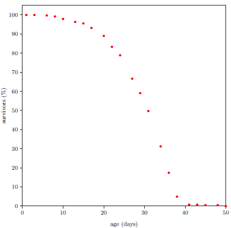A graph of the Figure 2.1 type is called a survival (or survivorship) curve. Survival curves show the percentage of survivors as a function of age for a population of organisms.

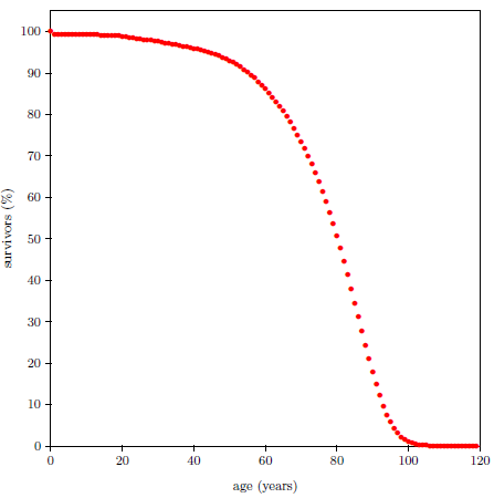
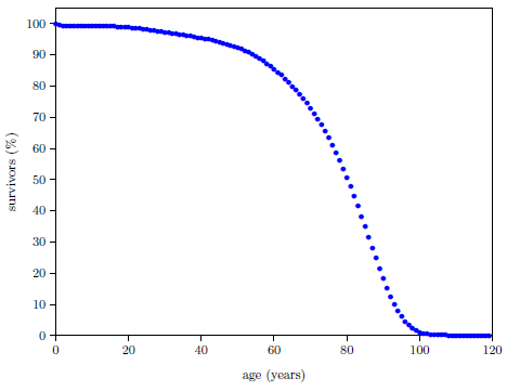
Survival curves can be plotted for all species, including humans. When we plot such a curve for humans today (Figure 2.2), we find that the shape of the curve is similar to that for fruit flies (Figure 2.1), even though the time axis is very different in the two cases. This ski-slope shape is, in fact, characteristic of well-cared-for organisms in general. It is definitive of aging. Specifically, the portion of the survival curve displaying increasingly rapid falloff with increasing age is what scientists have in mind when they talk about aging. In popular terms, this shape means that most individuals in the initial group live a "full" life before dying of modern human aging.

Figure 2.2: Survival curve data for modern U.S. males. (Data for this graph are for the year 2013 from the United States Social Security Administration's actuarial tables, located at ssa.gov/oact/STATS/table4c6%5F2013.html.)

2.4.2  The Gompertz Function

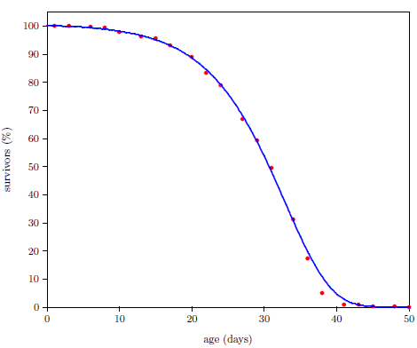
Survival curves are generally reasonably well characterized mathematically by a Gompertz function. This function has the (differential) mathematical form:

where N is the number of survivors at time t, K₀ is a proportionality constant, e signifies the natural exponential function, and A₀ is an exponential growth constant.

A few simple observations help give insight into the meaning of this equation. First, the left side of the equation, dN/dt, represents the number of individuals dying per unit time. It is just the death rate at any given time. The minus sign on the right side of the equation shows that the number of survivors decreases with time. Also on the right side of the equation, notice that at any time, t, the death rate is proportional to N, the number of survivors at that time. This is as it should be, of course. If one doubles the number of individuals in the group, then the number of individuals dying per unit time (the death rate) should also double.

The significance of the constant K₀ can be clarified as follows. The probability of death in a given time interval is defined as the number of individuals dying during the time interval divided by N, the number of individuals at the start of the interval. The number of individuals dying in the time interval is just N - N_final, where N_final is the number of individuals surviving at the end of the time interval. By definition of the differential, this is -dN. Thus, the probability of death is -dN/N. In the present case, this probability can be found by simple rearrangement of Equation 2.1.

At t=0, this equation reduces to K₀ = (-dN/N)/dt. The constant K₀ is thus seen to specify the probability of death of an individual per unit time at t=0.

Finally, the e^A₀t part of the right side of Equation 2.1 says that the probability of death per unit time increases exponentially with time. This is made explicit by Equation 2.2. The constant A₀ controls how quickly the probability of death per unit time increases.

Equation 2.1 may be integrated to yield an expression for N as an explicit function of t. The result, for A₀ ≠ 0 is:

This is the Gompertz function in its integrated form. It can be used to model survival curves resulting from biological aging.

This equation is graphed as a blue line in Figure 2.3 (using N₀=100, K₀=0.001 per day, and A₀=0.159 per day) and in Figure 2.4 (using N₀=99.219, K₀=9.1 ×10^-5 per year, and A₀=0.0815 per year). The Gompertz function obviously does a good job of characterizing real experimental survival curve data. (It is not expected to do a perfect job in the present case because, among other things, the survival curve data shown contain an admixture of deaths not due to aging, such as deaths due to automobile accidents in the case of U.S. males.)

Figure 2.3: Gompertz function fit to survival curve data for fruit flies.

Figure 2.4: Gompertz function fit to survival curve data for modern U.S. males.

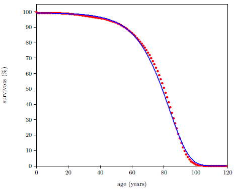While all the Gompertz function does, mathematically, is specify an exponentially increasing probability of death from birth on, this, nonetheless, results in a good characterization of real experimental survival curve data. This tells us that biological aging is characterized by an exponentially increasing probability of death from birth on. Now here is the critical question. Why should aging be characterized by an exponentially increasing probability of death from birth on?

2.4.3  A Thought Experiment

To find a rational answer to this question, perform the following thought experiment.

Imagine (leaving ethical questions aside) a cohort of a thousand peacefully coexisting modern young men, raised together since infancy on a desert island, with adequate shelter, but with no natural food supply. Airlift food and drink to them so they have a normal, balanced diet. When they reach age 25, withhold food but not water. Keep this up until the last of the thousand has died.

What will be observed, of course, in the weeks following removal of food from the diet, is an outbreak of the disease we call starvation. Since this disease is ultimately fatal when left untreated, it will eventually claim the lives of the entire cohort.

Figure 2.5 shows what may be expected. It shows survival curve data (red dots) for ten Irish hunger strikers who died of starvation.^[11] These ten hunger strikers were all males, ranging in age from 23 to 29. For the present purpose, which calls for a same-age group, the average age of the ten hunger strikers (25 years) has been used.

Figure 2.5: Survival curve for men due to starvation beginning at age 25 years.

The advent of starvation causes the mortality rate to begin to climb. Because human bodies are varied genetically, and because each individual's interaction with the environment is unique, cohort members do not all die at the same time. Some genetic constitutions will be more resistant to the ravages of starvation than others, and some individuals will experience less stressful interactions with the environment than others. But after a few weeks, individuals will begin to die of this disease. As time goes on, the probability of death will increase, and the longer time goes on, the more quickly the probability of death will increase.

Interestingly—tellingly—survival curve data for starvation can be characterized by a mathematical function very similar to the Gompertz function. The blue line in Figure 2.5 is a graph of the equation

using N₂₅=100, K₂₅=1.330 ×10^-3 per year (from the 2013 actuarial table data cited in Figure 2.2), and A₂₅=61 per year.

Notice that the blue line curve has the characteristic ski-slope shape. It looks very similar to the Gompertz curve describing aging. The only major difference is that it begins at age 25 years instead of at birth. In fact, Equation 2.4 reduces exactly to the Gompertz function of Equation 2.3 if 25 is everywhere replaced by 0 in Equation 2.4.

Like the Gompertz function, the kernel of Equation 2.4 is an exponentially increasing probability of death with time. This is shown more clearly by its differential form:

In Equation 2.4, the 25 is clearly specific to the case of the hunger strikers in question. In the general case, starvation can be initiated at any arbitrary age. Let T represent the age of onset of the disease. Then Equation 2.4 can be generalized as follows:

Starvation is just one example of a class of diseases characterized by Equation 2.6. It describes any disease having an exponentially increasing probability of death when left untreated. This is a large class of diseases. All nutritional deficiency diseases—for example, dehydration or scurvy or pellagra—belong to it. The class is not inclusive of all diseases, of course. Most infectious diseases—for example, chicken pox or the common cold—obviously do not belong to it.

Because T, the age of onset of the disease, may, in principle, be adjusted to any value, it may be adjusted to T = 0. When this is done, Equation 2.6 becomes the Gompertz function equation describing biological aging. Thus, the Gompertz function is seen to be merely a special case of Equation 2.6. Evidently, biological aging is indistinguishable from any exponentially progressing, ultimately fatal, universally present (i.e., present in all members of the population) disease which happens to be active starting at birth.

It might be felt that this is true only if one restricts the field of consideration to mathematics and survival curve shapes—that clinical symptoms could be used, for example, to differentiate between congenital disease and biological aging. But how? What clinical symptom is there which is uniquely and universally definitive of biological aging? The clinical symptoms of biological aging in fruit flies are significantly different from the clinical symptoms of biological aging in humans.

Biological aging is not defined by any set of clinical symptoms. In real life, it cannot be defined this way. Rather, it is defined "as an age-dependent or age-progressive decline in intrinsic physiological function, leading to an increase in age-specific mortality rate…"^[12] That is, aging is defined/diagnosed as a ski-slope survival curve starting from birth.

Any exponentially progressing, ultimately fatal, universally present congenital disease will give rise to "an age-dependent or age-progressive decline in intrinsic physiological function, leading to an increase in age-specific mortality rate." Thus, any such disease active in real life will simply be seen as and be called "biological aging."

Every indication, both mathematical/theoretical and clinical/experimental is that biological aging is indistinguishable from any exponentially progressing, ultimately fatal, universally present congenital disease. The simplest explanation of why this should be the case is that biological aging is, in fact, nothing more than exponentially progressing, ultimately fatal, universally present, congenital disease. This is just another way of saying that the essence of biological aging is congenital disease.

2.5  Conclusion

The essence of what we call "aging" in biology is simply congenital disease.

Chapter 3

Understanding the Etiology of Aging

The etiology—the root cause—of the phenomenon of aging is a matter of much confusion within mainstream science at present. Aging is ubiquitous within the biological realm. Its very prevalence seems to imply that biological evolution is itself the root cause of aging. Indeed, it is not uncommon to see trotted out the theory that evolution fosters aging to free up resources for the next generation once an organism's reproductive role has been fulfilled. Unfortunately, this notion butts heads with a basic tenet of evolutionary biology. Natural selection sees survival as a fundamental ingredient of evolutionary success (e.g., "survival of the fittest"), and aging accomplishes the opposite of survival. Evidently, the less fit are selected against by the very fact that they have lower survival. But this means that they have shorter life spans. And this says that natural selection selects for longer life spans. Meanwhile, aging acts to shorten life spans. Thus aging and natural selection are seen to act in opposite directions. How, then, can natural selection have brought about aging?

The General Theory of Aging for Biological Organisms remedies the current confusion. Rather than attempting to somehow reconcile the conflict between aging and natural selection, it embraces this conflict. Within its framework, natural selection, far from fostering aging, is seen generally to act against aging. Once it has been understood that congenital disease is the essence of aging, it then follows that the etiology of aging is to be found in whatever it is that occasions congenital diseases, and congenital diseases are found to be occasioned by imperfect design relative to existing environment—as I will now undertake to demonstrate.

3.1  A General Theory of Aging

The degree of complexity exhibited by even the simplest biological organisms makes elucidation of the etiology of aging difficult if discussion is restricted to the biological realm alone. To understand the etiology of aging, so as to be able to answer such basic questions as why aging is such a ubiquitous phenomenon in the biological realm despite the great diversity of biological organisms, it is helpful to extend the General Theory of Aging for Biological Organisms into the mechanical realm.

Biological organisms may be regarded as extremely complex biochemical machines. When the theory of aging is extended to encompass all machines, biological and mechanical, it becomes what I will call the "General Theory of Aging."

General Theory of Aging: Aging in all machines of all types is always simply progression of one or more disorders stemming from intrinsic design flaws relative to the machine's present environment.

Think about a fairly simple mechanical machine. For example, consider a small, two-stroke, internal combustion engine, such as might be used to power a weed eater. Imagine a cohort of a thousand such machines, all fresh from the factory. They are installed on identical weed eaters and put into constant use.

Two-stroke engines require that oil be mixed with the gasoline to lubricate their moving parts. Imagine that someone has forgotten this in the present instance so that all of the machines are being operated without oil. That is, imagine that a "disease state" has been induced in the machines by withholding oil. The moving parts of the engines wear with use (i.e., the engines age), and, after some hours, one after the other, the machines stop working (i.e., they die). Autopsy reveals that the piston rings have become too worn for adequate compression.

Plotting a survival curve for these engines is expected to yield a normal Gompertz function: the induced disease is present in the entire population of the machines, it is congenital, and the probability of death is expected to increase exponentially with time.

This is an example of mechanical aging. Aging in this particular instance of worn piston rings arises because of wear of moving parts. When metal surfaces rub against each other, atoms may be rubbed out of the contacting surfaces. These atoms may be lost from both surfaces, or they may move from one surface to the other, or they may relocate on one surface.

The disease which has been induced in these machines can be "cured" by addition of oil to the gasoline. Let us apply this cure to a second cohort of a thousand weed eater engines fresh from the factory. Repeating the above experiment, we find that the second cohort has a much longer average life span—months instead of hours. We have successfully cured oil deficiency disease, but we have not eliminated aging. Now a new cause of death emerges. Autopsy reveals that the spark plug electrodes have worn away, inhibiting the spark needed to ignite the fuel mixture. We have uncovered a new congenital disease of these engines: electrode ablation disease. This is not an induced congenital disease; rather, it is an intrinsic congenital disease, inherent in the present design of the machine.

A cure for this intrinsic congenital disease might be found by choosing a different metal for the electrodes, one which is better able to withstand the electric arc plasma (i.e., the spark) each engine cycle. This would give the machine an even longer average life span, but it would still not entirely eliminate aging. The cause of death might now be found to be due to the air filter slowly clogging, reducing air supply to the cylinder. This causes the spark plug to become fouled with soot, so it shorts out and no longer sparks. This congenital "pulmonary fibrosis" disease is interesting because it shows an example of aging which is not due to wear. The air filter is not worn. It just needs to be cleaned.

3.1.1  Longevity and Natural Selection

We have just seen that changes to the design of a machine can significantly alter its spectrum of congenital diseases and thereby impact its longevity. Biological organisms are mutable, self-replicating machines. Mutation alters machine design, creating diversity in offspring. Thus, longevity will vary in biological offspring. Longevity is a heritable trait. As such, it is subject to natural selection.

Longevity Principle

What effect does natural selection have on the longevity trait? My exploration of this question causes me to formulate the following simple Longevity Principle:

Longevity Principle: Successive generations of mutable, self-replicating machines tend to increase in longevity.

This principle may be empirically justified as follows. First, observe that there are only three possibilities. Successive generations of mutable, self-replicating machines may tend to:

1. decrease in longevity,
2. conserve longevity, or
3. increase in longevity.

Next, consider the long-term outcome of each of these three possibilities:

1. Self-replicating machines tending to decrease in longevity from one generation to the next will eventually go extinct.
2. The only way to leave longevity unchanged long term is for there to be equal probability for longevity to trend either up or down on the short term. The statistics of the well-known random-walk-near-a-cliff problem assure us that this case, too, will end in extinction.
3. Only self-replicating machines tending to increase in longevity from one generation to the next are able to go on propagating indefinitely.

Finally, observe that there exists but one known experiment on this at present. This is the natural experiment involving mutating, self-replicating organisms on earth. Scientists report fossils of microorganisms in rocks with measured ages of 3.5 billion years. Though the experiment appears to have been running for 3.5 billion years, in all this vast expanse of proleptic time the predicted outcome of the first two possibilities—universal extinction—has not been realized. Rather, what is presently observed is existence of a plethora of long-lived (i.e., months, years, decades, centuries, and even millennia) organisms. Thus the Longevity Principle—that successive generations of mutable, self-replicating machines tend to increase in longevity—is seen to work in this solely available instance.

This empirical justification may be augmented by a simple theoretical justification. Mutable, self-replicating machines produce offspring varying in their ability to stave off death. Offspring best able to stave off death have more time in which to produce and raise offspring. Hence, those mutable, self-replicating machines which are best able to stave off death are likely to leave more offspring. As a result, the machine population will shift with time toward machines which are better able to stave off death. Thus, longevity is naturally selected for, causing successive generations of mutable, self-replicating machines to tend toward increasing longevity.

3.1.2  Impediments to Increasing Longevity

Though the Longevity Principle states that the trend from generation to generation is to increase in longevity, it is clear that this trend will not be linear in the general case. It is also clear that the incremental change in longevity with time is unlikely to be monotonic. Two obvious impediments to increasing longevity are increasing complexity and changing environment.

Increasing Complexity

Remedies for congenital diseases generally entail increasing complexity, but increasing complexity increases the number of potential congenital diseases.

For a four-stroke internal combustion engine, the problem of frictional wear of parts is alleviated by the machine itself pumping oil to moving metal joints. This frees the operator from having to remember to mix oil with the gasoline. Once again, the lubrication of rubbing metal surfaces greatly increases the longevity of the engine relative to an unlubricated engine. But this method of lubrication also significantly increases the complexity of the engine. To implement engine self-lubrication, necessary additional parts include an oil reservoir, an oil pump, and an oil filter. Each of these parts has potential to fail and cause death of the engine. Thus, while adding the self-lubrication functionality increases engine longevity, it also adds more potential congenital diseases, making further gains in longevity comparatively more difficult to achieve.

Changing Environment

Environmental changes can lead to large losses in longevity.

In the mechanical machine realm, this is analogous to loss of lubricating oil from the four-stroke engines' environment. Since the engines do not make oil, oil must be supplied to the engines' oil reservoirs from the external environment. In an environment in which oil is faithfully supplied, the machines have no intrinsic design flaw in this regard. But, if the environment changes in such a way as to cut off supply of oil to the engines, leaving the oil reservoirs of new engines empty, then the engines will revert back to their much shorter unlubricated longevity. The changed environment has created an intrinsic design flaw—lack of lubrication—which results in a sudden loss in longevity.

3.2  Conclusion

According to the General Theory of Aging presented here, imperfect design relative to the existing environment gives rise to congenital diseases, one or more of which dominates, progressing with age and ending ultimately in death. The greater the complexity of a machine, the more ways there are for things to go wrong. Because even a single-celled organism displays extreme complexity, the potential for congenital diseases with biological organisms is clearly enormous. Hence the ubiquitous presence of aging in biological organisms.

Fortunately, the potential for cures is also much greater biologically than it is mechanically. We have seen that adding oil to the gas of a two-stroke engine reduces wear between moving parts but does not completely eliminate it. Eventually, wear will cause the engine to die, even with adequate oil present at all times. The ideal cure for wear would be for the machine to have a way of putting displaced atoms back where they belong. While it is difficult to see how this might be accomplished with present mechanical machines, it is not at all difficult to see how it might be accomplished with biological machines. Biological machines operate at the molecular level. They have theoretical potential to renew parts continually, molecule by molecule. And indeed, such repair mechanisms do exist within biological machines. Cellular self-repair of double-stranded DNA is one such example.

For mutating, self-replicating machines, mutation occasions both design improvements and concomitant novel imperfections. Natural selection is ever in the process of eliminating these imperfections, one congenital disease after another. If natural selection were allowed to act for an infinite time in a static environment, then all congenital diseases might be eliminated and immortal machines result. But this would be the final end point. The starting point is at the other end of the scale, populated by very mortal machines.

Earth's biosphere, in its present form, exists somewhere between these two termini. We learn from the historical sciences that earth's environment has been far from static. Nonetheless, earth's biota has clearly progressed a considerable distance along the longevity scale, sporting some species, such as the bristlecone pine (Figure 3.1^[13]), having life spans measured in thousands of years. And, according to the Longevity Principle, we should not regard earth's biota, including humans, as now static in regard to longevity, but rather as progressing toward yet greater life spans.

Figure 3.1: Bristlecone pine tree, White Mountains, Nevada.

Chapter 4

Modeling Survival Curves in Light of the General Theory of Aging

The cause and the cure of modern human aging presented in this book is dependent upon analyses of human survival curve data, both ancient and modern. The General Theory of Aging sheds new light on survival curves, and this affects how they should be analyzed. The method that will be used to analyze survival curve data throughout the remainder of this book needs to be explained at this point. Consequently, this chapter is devoted to technical material which many lay readers may want to skip over. There is no harm in doing so.

4.1  Data Analysis Method

Figure 4.1 shows survival curve data for U.S. males. These data are for the year 2016 from the United States Social Security Administration's list of actuarial tables.^[14] These 2016 data will be used in the following pages to illustrate the least-squares data analysis method which the General Theory of Aging prompts.

Figure 4.1: Survival curve data for modern U.S. males.

4.2  The Model

Traditionally, the Gompertz function has been used as a model for survival curve data. The General Theory of Aging reveals that this function is not entirely right for the job.

The Figure 4.1 survival curve is clearly dominated by aging. That is, most of the deaths are due to aging. That is why the number of survivors falls off so rapidly after about age 60—modern human aging is killing nearly everybody off.

While aging is the dominant cause of death, it is not the sole cause of death. The data of Figure 4.1 contain an admixture of deaths not due to modern human aging. For example, infant mortality is noticeable in the very first year of the graph. Less conspicuous, but equally real, are deaths due to traffic accidents. In fact, there are deaths due to hundreds of causes other than modern human aging in this dataset: everything from homicides to lightning strikes.

Let us call deaths which are not due to aging, "extraneous" deaths. The Figure 4.1 graph is made up, then, of two components: (1) deaths due to the congenital aging disease(s) and (2) extraneous deaths.

The Gompertz function is, in general, not well suited to describing extraneous deaths. We have previously seen that the Gompertz function describes an exponentially increasing probability of death per unit time with calendar age. There is no reason why the probability per unit time of being struck by lightning should increase exponentially with the calendar age of the individual being struck. Does a 40-year-old have a much greater chance of being struck by lightning than a 20-year-old, and does a 60-year-old have a yet much greater chance of being struck by lightning than a 40-year-old?

The Gompertz function is an approximation only. It smears together many independent causes of death, most of which are not expected to be exponentially increasing with age. The Gompertz function gets away with this wherever the survival curve is dominated by deaths due to aging because the aging disease is characterized by an exponentially increasing probability of death per unit time, as we have previously seen.

Mathematically, at least two terms are required to describe what is really going on with real-life survival curve data. One term is needed to describe deaths due to aging, and another term is needed to describe extraneous deaths.

It might be thought that what is needed, then, is (1) a Gompertz function to describe deaths due to aging, and (2) some other function to describe extraneous deaths. But, as it turns out, the Gompertz function doesn't describe aging deaths quite properly either. The Gompertz function happens to be a workable approximation for aging deaths, but it is not quite right.

The General Theory of Aging clarifies that aging is exponentially progressing congenital disease. In developing the General Theory of Aging, two-cycle engines were used to illustrate possible "congenital diseases" leading to "death" of the machines. Lack of lubricating oil leading to wear of piston rings and consequent loss of compression was given as one example. Ablation of the spark plug electrode was given as a second example. And clogging of the air filter was given as a third example.

Taking these three cases as representative of general aging diseases, notice that they all require some passage of time before the first death appears. For piston rings to wear sufficiently for the machine to become inoperable, the machine must be operated for some amount of time. For the spark plug electrode to wear away by ablation, some finite number of sparks must be generated, and this means that the machine must be operated for some amount of time. For the air filter to become clogged, air must be pulled through it, and this means that the machine must be run for some amount of time.

For these three examples, there will be no deaths due to these aging diseases when the machines are new. Said more precisely, the rate of death of these machines due to each of these three aging diseases when the machines are brand new is zero.

This seems to be a general property of aging diseases. It seems intuitive that the initial probability of death due to aging must be zero since initially (i.e., at t=0) there has not yet been any aging.

Curiously, the Gompertz function, which otherwise describes aging so well, does not allow the initial rate of death to be zero.

The Gompertz function has the differential form:

In this equation, t is the time (generally specified as the age of the organism for survival curves), N is the number of individuals surviving at time t, dN/dt is the population growth rate (the negative sign in the equation says that the population is shrinking in this case, due to deaths), K is the probability of death per unit time at t = 0, and e^At specifies an exponential increase in the probability of death per unit time, the rapidity of which is controlled by A.

At t = 0, Equation 4.1 reduces to:

This is the initial rate of death, and it is not zero. N₀, the initial number of machines, is not zero, of course. K is also not zero. Equation 4.1 shows that if K were zero, then the rate of death would always be zero for all time. This means that there would be no death and no aging, and all machines would go on living forever. For aging to be present, K cannot be zero. Thus, neither N₀ nor K is zero, and this means that the Gompertz function excludes the very real case of the initial rate of death being zero for an aging disease.

Thus, surprisingly, the Gompertz function is found to describe properly neither death due to aging nor extraneous deaths.

Why, then, does the Gompertz function do a good job of describing real-world, aging-dominated survival curves? It is because it smears together aging deaths and extraneous deaths, and extraneous deaths can reasonably have a non-zero rate of death at t=0. There is, for example, no need for any passage of time for a lightning strike to cause a death. A lightning strike can kill a brand new machine the instant it comes off of the assembly line.

When aging deaths and extraneous deaths are separated out, the Gompertz function is no longer useful. We very much desire to separate aging deaths from extraneous deaths because we wish to study aging specifically, not deaths in general. When studying aging specifically, extraneous deaths act as a background interference, obscuring what we are trying to learn about. It is, therefore, necessary to part company with the Gompertz function at this point.

4.3  Beyond Gompertz

Having bid a nostalgic farewell to the Gompertz function, we now find ourselves in need of a function which properly describes aging deaths. As it turns out, a suitable function can be obtained by a modification of the Gompertz function. The right side of Equation 4.1 can be made to be zero at t=0 as follows:

This equation is no longer the Gompertz function. It is distinctly different from Equation 4.1, which defines the Gompertz function. A retains its meaning, as the exponential growth constant, but the meaning of K is changed. It is no longer the probability of death per unit time at t=0. For Equation 4.3, the probability of death per unit time at t=0 is, by design, zero. K is now simply a proportionality constant, acting as a "gain" control for the exponential increase from zero of the probability of death per unit time.

While Equation 4.3 is no longer the Gompertz function, it retains everything the Gompertz function does correctly in regard to aging and adds in the benefit of having a zero rate of death at t=0. It will be utilized in place of Equation 4.1 to describe aging deaths from now on.

To describe real-life survival curve data accurately, we need also a function which describes extraneous deaths. The rate of extraneous deaths is obviously complicated. For humans, it will be different in a time of war than during peacetime, for example. Extraneous deaths can have many different causes and, consequently, many different functional forms.

A general approach in such a case might be to use a Taylor series to approximate the function describing the rate of extraneous deaths. This gives:

I have found that dropping all but the first term in this series works well in practice for lab data. One expects this to work well in practice because, for controlled laboratory survival curve data, one chooses experimental conditions deliberately to minimize extraneous deaths, and the strong (i.e., exponential) time dependence of death due to aging is expected to kill off the population before higher order, t-dependent terms in Equation 4.4 can grow large enough to have much impact on the death rate.

This gives as an approximation for the rate of extraneous deaths:

In this equation, R specifies a constant probability of death per unit time due to extraneous deaths. This approximation finds considerable support from its long-standing use within the Gompertz–Makeham law of mortality, where it supplies the Makeham term.

The equation describing real-life survival curve data in this approximation, combining both deaths due to aging and random extraneous deaths (i.e., those having a constant probability of occurrence, independent of time), is then:

In this equation, as K increases, the death rate due to aging increases, and as R increases, the death rate due to random extraneous deaths increases. The solution of this differential equation is:

This is the model which I will start with in all that follows. I will call it the "Aardsma model" to be clear that we are no longer using the Gompertz function.

Notice that this model takes into account only one congenital aging disease. Additional terms are needed in the model if two or more congenital aging diseases are present having nearly equal dominance. In practice, one expects only a single congenital disease to show up at a time in most cases because the exponential increase in death rate due to the most dominant aging disease is likely to have killed off the population before the next most dominant congenital disease has begun to have much of an effect on the death rate.

Notice also that, in this approximation, the total rate of deaths separates into a time-dependent component (due to aging deaths) and a time-independent component (due to a constant background of "noise" deaths).^[15] "Noise" deaths are due to random events like lightning strikes. Thus, the model's applicability is limited to survival curves where extraneous deaths are due to random events. Rather than calling these "random extraneous deaths," I will use the shorter "random deaths" to mean the same thing from now on.

4.4  Weighting the Fit

Survival curve data points do not all have the same measurement uncertainty. As a result, it is necessary to weight the data points to obtain the optimum fit of the model.

In any survival curve experiment, the fundamental observation is the number of deaths in a time interval. For the actuarial life table data of Figure 4.1, the data points are for one-year time intervals, each interval corresponding to a given age. The number of deaths which occurred in each age interval can be obtained from the actuarial table. For example, the 2016 actuarial table shows that, for a total of 100,000 males dying in 2016, 230 died in their 41st year (i.e., between their 40th and 41st birthdays), and 462 died in their 51st year.

These numbers of deaths are not to be taken as exact. Imagine breaking the total number of U.S. males who died in 2016 (roughly 1,400,000) into randomly chosen groups of 100,000. The number of deaths in the 41st year age interval would not be exactly 230 for every one of these groups. Basic counting statistics teaches that the number of events counted from group to group will fluctuate as the square root of the average for that age interval. This means that the 230 of the 41st year is to be treated as 230 ± 15.2 deaths, and the 462 of the 51st year as 462 ± 21.5 deaths.

This illustrates that varying measurement uncertainties are associated with the number of deaths corresponding to each age interval. When carrying out a least-squares fit of a given model to measured data, it is intuitive that data points having less uncertainty should be given relatively more weight in determining the optimum values of the model's parameters (i.e., A, K, and R in Equation 4.7 for the Aardsma model). A weighted least-squares analysis is, therefore, required. This is accomplished in the usual way, by assigning each data point a weight equal to the square of the reciprocal of its uncertainty.

Error bars depicting the size of the uncertainties associated with each data point are normally displayed graphically with the data. In the present case of the 2016 actuarial data, the error bars are too short to be visually discerned on the graph. The error bar for the 51st year, for example, plots as a vertical line through the data point at x=50.5 years and y=91.747 percent survivors. Its length is much too short to be seen on the graph, just (2×21.5/100,000×100=) 0.0430%.

For usual lab experiments, the number of experimental animals used is much smaller than the number of males included in the 2016 actuarial life table, and this results in much larger error bars which are generally easily discerned graphically.

4.5  Performing the Least-Squares Fit

It is necessary to use a computer to carry out the mathematical computations needed to perform the least-squares fit. Algorithms for this task have been around for a long time and do not need to be coded from scratch. I have used functions (FCHISQ, FUNCTN, and FDERIV) and subroutines (CURFIT and MATINV) written by Bevington in Fortran IV and published in 1969.^[16] Both FUNCTN and FDERIV were adapted by me, as intended by Bevington, to suit the present model. A listing of a program I wrote for this purpose can be found in Appendix A.

4.5.1  Post-fit Scaling of Uncertainties

When a weighted least-squares fit of the Aardsma model to the 2016 actuarial life table data for males is carried out, the fitted curve shown in Figure 4.2 results. (I have excluded the first data point from this fit because the large infant mortality it reflects is not included in any way in the Aardsma model.) The fit is visibly good (not great), but the goodness-of-fit parameter, reduced chi-square (Χ_ν²), has a value of 1316, which says that the fit is statistically extremely poor. For a good fit, Χ_ν² is expected to be near 1.

Figure 4.2: Survival curve data for modern U.S. males (blue) with least-squares fit of the Aardsma model (red).

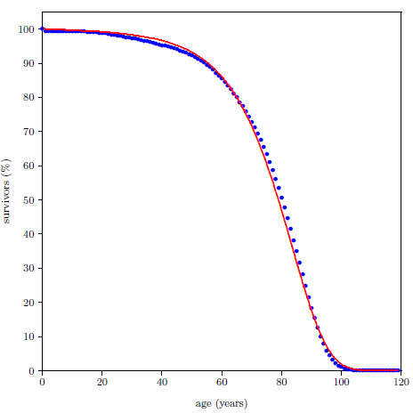The large value of Χ_ν² in this instance is not characteristic of normal laboratory survival curve data. It happens because the fit, in this instance, is extremely poor. Visually, it looks not all that bad, but relative to the (microscopic) error bars on the data points, it is terrible. For such tiny error bars, the fitted curve resulting from a good fit would be seen to pass through the approximate center of each blue data point on the graph. The least-squares fit curve does not do this. It is visibly off center much of the time.

The reason the fitted curve doesn't pass through the centers of the data points is because the Aardsma model does not adequately describe all that is going on with this survival curve. The Aardsma model undertakes to explain only two kinds of deaths in this data set, just random deaths and deaths due to aging. These two kinds of deaths explain a great deal of what is going on with this data set, but they do not explain everything. Because the Aardsma model does not describe infant mortality, I excluded the first data point from the fit, as mentioned above. To include infant mortality in the model, another term would need to be added to the differential rate of death equation (Equation 4.6). But, as there is a lot more than just infant mortality going on with the extraneous deaths in this data set, many more terms are needed for a complete description. For example, notice that beginning around age 20, the data points begin to fall noticeably below the fitted curve. By roughly age 35, the data points (represented by blue dots having diameters much larger than their error bars in all cases) and the fitted curve are barely even touching one another. This says that there is a systematic loss of young men from this survival curve which has nothing to do either with aging or with random deaths. And indeed, according to the Center for Disease Control and Prevention (CDC), for the year 2016, 13.4% of deaths in the 20–44 years age range were due to suicides, 9.6% were due to homicides, and another 1.0% were due to HIV disease.^[17] The Aardsma model includes none of these extraneous deaths.

Here again this 2016 actuarial survival curve for U.S. males is seen to be different from controlled laboratory experimental survival curves. The sorts of extraneous deaths it involves do not generally present themselves in lab experiments. Neither mice nor fruit flies use guns lethally or commit suicide, for example. But this survival curve does a very good job of teaching some of the finer points of modeling survival curve data sets via least-squares, which is why I have chosen to use it in this chapter.

The goodness-of-fit, Χ_ν², can be improved by increasing the uncertainties in the individual data points. This is a deliberate workaround, having no other purpose than to approximate more accurately the uncertainties in the fitted model parameters A, K, and R. In effect, this workaround shifts the blame for the poor fit over to the uncertainties in the data points, saying that they are unrealistically too small. In reality, of course, it is the model which has the problem. It has too few terms to describe what is really going on with the data set. By expanding the data points' error bars, all by a constant factor, we bring the data into closer harmony with the model by making the fine structure in the data, due to extraneous deaths, become small relative to the (inflated) uncertainty in the data points.

This workaround does not affect the values of the fitted parameters in any way. Only their estimated uncertainties are affected. Multiplying all error bars by a constant factor does not change the relative weights of the various data points, so the final fit is the same. Again, the reason for expanding the error bars to get a better goodness-of-fit value is purely to obtain more realistic estimates of the uncertainties in the final parameters from the available dataset. Expanding the error bars on the data points by a constant factor increases the estimated uncertainties in the fitted parameters by the expansion factor.

In practice, this workaround is implemented automatically by the computer program in all cases. The factor by which the uncertainties of all the data points need to be multiplied to obtain Χ_ν² = 1 is just the square root of Χ_ν². Thus, the computer program merely multiplies the estimated uncertainties in the parameters by the square root of Χ_ν² at the conclusion of the least-squares analysis. For the 2016 actuarial male survival curve, this workaround increases the estimated uncertainties in the fitted parameters by a factor of 36. For laboratory survival curve data, this workaround generally results in a much more modest (10 or 20 percent) adjustment of the estimated uncertainties of the parameters.

4.6  Separation of Signal from Noise

Because the Aardsma model cleanly separates deaths due to the aging disease from random deaths, it allows these two contributions to the survival curve data set to be studied in isolation from each other. The least-squares estimated survival curve due to aging alone results from setting R to zero in Equation 4.7 while otherwise using the values for A and K found by the least-squares fit. Similarly, by using the value for R found by the least-squares fit in Equation 4.7 while setting K to zero, the least-squares estimated survival curve due to random deaths alone results. These two cases are shown in Figure 4.3.

Figure 4.3: Survival curve data for modern U.S. males (blue dots). The least-squares fit of the Aardsma model is shown in red. Orange shows the model's estimated survival curve in the absence of aging, and green shows its estimated survival curve in the absence of random deaths.

4.7  Conclusion

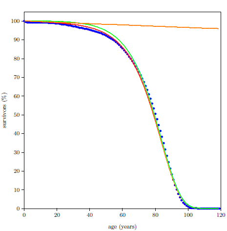The Gompertz function, Equation 4.1, is found not to describe adequately survival curve data which include aging deaths. To describe such data, the function shown in Equation 4.3 is used in the present work.

For researching biological aging, much laboratory survival curve data can be adequately modeled by adding to the foregoing function a time-independent random death term as shown in Equation 4.6. This is called the "Aardsma model" in the present work. In its integrated form, the Aardsma model appears as shown in Equation 4.7.

A weighted, least-squares fit of the Aardsma model in its integrated form (Equation 4.7) can be made directly to survival curve data. In the case of multiple congenital diseases present within the studied organism, the model can be expanded to include more than one aging disease term. For two aging diseases, for example, the model becomes:

This allows the various contributions to survival curve deaths to be separated out and studied independently of one another.

Chapter 5

The Biblical History of Human Aging

5.1  Life Spans

My research into aging breaks with other contemporary scientific research on aging in its attitude toward the life span data found in the earliest books of the Bible (Table 5.1). These data, because they sport human life spans of hundreds of years—in some instances approaching nearly a thousand years—are commonly held to be mythological by contemporary researchers. The attitude toward these data underlying my work is opposite to this. I hold these data to be valid, accurate, invaluable, historical observations of actual life spans of real individuals.

Table 5.1: Selected biblical life span data.

This attitude is neither arbitrary nor religiously biased. The idea that these data are mythological or otherwise concocted cannot be retained by any scientist who has actually worked with them. These biblical data display certain features which are impossible to explain in any other way than that they are valid historical observations. This property will become increasingly clear as we proceed through this book. For now, I simply point out that the basically historical nature of these life span data is already strongly implied by their intimate association with key biblical chronological data. Many of these life span numbers are recorded together with birthdate numbers which are used directly in the construction of the chronology of biblical history stretching back to Adam. When this biblical chronology is checked using radiocarbon dating, it is found to be remarkably accurate. For example, the biblical chronology date for Noah's Flood is 3520±21 B.C., and the corresponding radiocarbon date is 3525±12.5 B.C.^[18] This is probably the most secure and precise date humankind possesses for any historical event of such remote antiquity. The biblical chronological numbers are demonstrably historical. Would it not be odd if the closely associated life span numbers were mythological?

Once the biblical life span data have been accepted as historical and reliable by any scientist researching the cause of aging, they automatically become his central focus. They necessarily do so because they report on a unique, real-life, natural historical "experiment" which displays a pronounced life span effect in humans. Life spans start out near 1,000 years, but then decline, reaching modern levels for individuals subsequent to Moses. This is the only experimental evidence we have that the modern human life span is mutable. Experimental data displaying any evidence for even the slightest extension of the present human life span are of extreme interest, but the Genesis longevity data go far beyond this, displaying evidence that human life spans may be extended by more than a factor of ten. Obviously, the biblical historical life span data are of unparalleled value to any truly scientific effort to solve the mystery of modern human aging.

Though the Table 5.1 list is comprehensive, it is not exhaustive. To begin with, biblical individuals with anomalously low life spans, such as Enoch (Genesis 5:24), Lamech (Genesis 5:31), and Nahor (Genesis 11:24–25) have been excluded. Secondly, biblical females have also been excluded. Males and females have different average life expectancies, so they need to be treated separately. There are significantly more life span data points for biblical males than there are for biblical females, so the present study focuses much of its attention on male life spans, both ancient and modern. Finally, no attempt has been made to add data to the list after Moses. Such data are of limited interest in the present study. They show mainly a continuation of the roughly 75-year average life span which, on the basis of Psalm 90 ("A Prayer of Moses the man of God"), was already operative by the time Moses died.

Despite these exclusions, the list presents a remarkable dataset. Its 26 data items clearly capture a remarkable decline in human longevity in the past.

5.2  Birthdates

The Table 5.1 life span data are everything. Understanding why they declined as they did is the goal. It is not sufficient simply to observe that life spans were longer in the past. The goal is to discover why they were longer—what physical, material agent(s) caused human life spans to shorten. The goal is to elucidate a cause and effect relationship. To accomplish this, knowledge of how life spans changed with time is needed. Thus, to make full use of these life span data, it is necessary to attach a unique time to each data item, specifying when in history that particular life span applied. This can be accomplished by assigning proper calendrical birthdates to each of the individuals listed in the table. If it is then assumed that each of the individuals shown in the table died of aging, then the life spans of these individuals can be used as an estimate of the aging-specific life expectancy when they were born. This will allow a graph to be constructed of life expectancy versus time for the ancient past, which is what is needed to attack the problem of the specific causes of reduced human longevity quantitatively.

Table 5.2 shows the needed birthdates. These dates have been computed from a combination of both biblical and extra-biblical chronological data according to the principles of the modern discipline of biblical chronology. The "Chronology Numbers" column shows numbers which are needed in the computations of the birthdates, and the "Bible Reference" column shows where these numbers were obtained.

Table 5.2: Birthdates of selected biblical males.

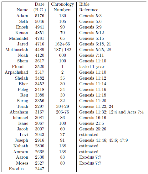The table includes two chronological reference points: Noah's Flood at 3520 B.C.^[19] and the Israelite Exodus from Egypt at 2447 B.C.^[20] The date of the Flood is used as the reference point for most of the dates in the table, but chronological continuity, provided by recording the age of the father at the birth of the son, is lost following Jacob, during the 450 years Israel was in Egypt, making the final six birthdates of the table somewhat more complicated to compute.

The birthdate of Joseph can be calculated using the three Bible references provided for Joseph in the table. These reveal that Joseph was 39 years old when Jacob was 130 years old. Thus Jacob was 91 years old at the birth of Joseph.

Levi's date of birth has been estimated from Joseph's date of birth by making use of the fact that Joseph was the ninth son after Levi. Natural child spacing tends to be about three years (compare Moses and Aaron, for example) yielding 27 years between Levi and Joseph. This simple means of estimation is called into question in this instance by the fact that four separate wives were involved. This potential complication has been ignored since, from the primary record found in Genesis 29 and 30, the births seem to have been consecutive rather than overlapping, and because even a crude estimate will suffice for the present purpose.

For calculating the dates of birth of Moses and his brother Aaron, the date of the Exodus must be used. Exodus 7:7 reveals that Moses and Aaron were 80 and 83 years old respectively when they confronted Pharaoh. This places the birth of Moses in 2527 B.C.

The birthdates of Kohath and Amram can only be estimated. Even a crude estimate will suffice here once again, because life spans were not changing very rapidly when Kohath and Amram lived. Kohath and Amram have simply been placed equally apart in the 413-year interval spanned by the father-son lineage, Levi–Kohath–Amram–Aaron.

5.3  Life Expectancy

Life expectancy is the length of time a person may be expected to live. Since the current study is concerned with human longevity, it is the life expectancy at birth which is of interest. For the current study, life expectancy at birth data are obtained by combining the age at death data from Table 5.1 with the birthdate data from Table 5.2. The result is shown in Table 5.3.

Table 5.3: Point estimates of life expectancies from Adam to Moses.

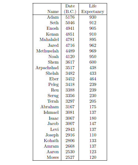Normally, life expectancies are calculated by averaging ages at death from a large population. The biblical life span data provide only individual data points, not averages over many individuals. This is the same as taking the age at death of a single randomly-chosen modern male to estimate the life expectancy at birth of modern males worldwide. While the average life expectancy is likely to be near 75 years at present, not all males die at age 75 years. Instead, ages at death of, for example, 62 years or 87 years are quite common. Individual ages at death today can easily differ from the average by plus or minus twenty years. The same is true of the biblical life expectancy data points. In fact, the average life expectancy at birth of the first seven individuals in the table, taken from a time interval during which life expectancies are thought to have been more or less stable, is 926 years, with a standard deviation of plus or minus 28.9 years.

5.4  Conclusion

Figure 5.1 shows a graph of these biblical data. Take a good look at it. There is no graph in the whole world of greater practical humanitarian importance than this one. It is the key which unlocks the mystery of the cause and cure of human aging, as subsequent chapters will show.

Figure 5.1: Biblical data showing life expectancy at birth for selected males.

Chapter 6

The Biblical Life Expectancy Graph

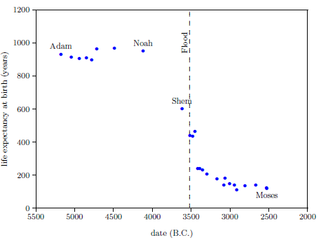Before beginning to apply the data displayed in Figure 5.1 to solving the mystery of human aging, it seems appropriate to point out two unique advantages from which the present research has benefited.

The first unique advantage has been the ability even to construct this graph. To construct this graph, one has to have one's biblical chronology right all the way back to Adam. Most importantly, as will become increasingly clear, one has to have the date of the Flood right. The key to these prerequisites is the recognition that traditional biblical chronology has dropped out a full millennium in 1 Kings 6:1.^[21] This discovery was made only in 1990. Extension back to Adam of the new biblical chronology resulting from that discovery was not completed until 1999.^[22] Thus, though the biblical life span data of concern to this study are of great antiquity, ability to plot them accurately on the graph of Figure 5.1 is little more than two decades old.

In addition to having biblical chronology right, the research reported in this book enjoyed a second important advantage. Figure 5.1 shows plainly that Noah's Flood is the dividing line between the short life span regime of the present day and the long life span regime of the ancient past. The reduced life expectancy data point corresponding to Shem, just before the Flood, may seem to be an exception to this, but Shem's reduced life span results from the fact that he lived most of his life in the post-Flood period. He was born 97 years prior to the Flood, and he died 503 years after the Flood.

The observation that Noah's Flood is the dividing line between the ancient and modern longevity regimes implicates Noah's Flood as the fundamental cause of reduced life spans today—the cause of modern human aging. Noah's Flood appears to have done something which subsequently shortened human life spans causing modern human aging. What exactly did it do? This is the fundamental question which must be answered in seeking to solve the cause of human aging.

Clearly, to have any hope of answering this question, an accurate idea of the nature of the Flood is needed. Indeed, the paramount importance of an accurate knowledge of the nature of the Flood to cracking the mystery of the cause of human aging will become increasingly apparent in subsequent chapters. For now, the point to notice is that the true nature of the Flood was discovered only in 1997.^[23]

Thus, both of the ingredients needed to make quantitative, scientific sense of the biblical life span data—a correct biblical chronology and a correct understanding of the nature of the Flood—have become available only since 1998.

These two unique advantages did not guarantee, of course, that this ancient mystery could, at long last, be solved. But they did make it perfectly clear that the time had come for a new, all-out assault on the problem.

6.1  A Powerful Instrument

The Figure 5.1 graph is a powerful research instrument. Consider its application in the following four cases, the first three dealing with mistaken theories of aging and the fourth dealing with the General Theory of Aging presented in chapters 2 and 3.

6.1.1  Supernatural

Perhaps the simplest lay theory of aging is that the human life span is determined by God in ways that cannot be understood or ascertained by humankind. This denies any natural cause of aging, which immediately yields the corollary that scientific investigation into the matter is useless.

The biblical life expectancy data argue strongly against this theory. They show that human life spans declined in a fairly smooth way from roughly 930 years on average before the Flood to roughly 75 years on average following the Flood. This smooth decline took more than a thousand years to settle out to the currently active average life span. If the human life span is fixed by God, then these data require that God performed numerous miracles, continuously readjusting human life spans for more than a thousand years following the Flood. This seems severely contrary to what we learn of the nature of God's supernatural activity elsewhere in the Bible. Based on the miracles we read about in the Bible, such as the conversion of water into wine (John 2:1–11), or the calming of the sea (Luke 8:22–25), or the iron axe head which was made to float on water (2 Kings 6:1–7), we expect miracles to be generally evidenced as point-in-time suspensions of the natural order, not as innumerable slight adjustments of the natural order.

Meanwhile, we expect natural processes to change smoothly with time. For example, the temperature of a bowl of hot water naturally changes in a smooth progression from hot to cold with time (Figure 6.1).

Figure 6.1: Measured temperature versus time for a bowl of hot water.

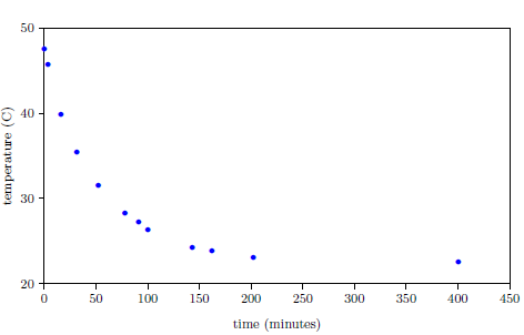Furthermore, the change in temperature of the hot water is more rapid at first, and slows as it nears room temperature. This property is seen in the biblical life span data as well: the rate of change of life spans is rapid immediately following the Flood and slows as the present value near 75 years is approached.

The biblical life span data reveal that life spans declined in a natural way following the Flood, implying that some natural cause was responsible for this decline.

6.1.2  Vapor Canopy

A second lay theory is that pre-Flood longevity was due to a water vapor canopy which enveloped the earth prior to the Flood. This canopy was supposedly suspended above the atmosphere before the Flood, but it condensed and fell to the earth as rain at the time of the Flood, thereby contributing to the Flood's forty days and nights of rain.

This vapor canopy theory was popular a few decades ago with some people who regard Genesis as historical. Today, it is generally discredited. A scientific explanation of how such a canopy of water vapor might be kept in place is lacking. What would keep the water molecules from mixing with the rest of the atmosphere? Notice that the atmosphere today does a very good job of mixing all of its constituents together. We do not find separate layers of oxygen, nitrogen, carbon dioxide, water vapor, or any other gas. Other serious scientific problems a vapor canopy introduces include greenhouse heating of the surface of the earth and inordinate heating of the atmosphere at the time of the Flood due to the heat of condensation of water vapor and the conversion of gravitational potential energy to heat energy which would result from collapse of such a canopy. The only reason for bringing it up here is to show the power of the biblical life expectancy data for falsifying mistaken theories of aging.

The canopy is credited by its adherents with prolonging life prior to the Flood, usually in one of two ways. The first is through attenuation of hypothetically harmful radiation from space. Some versions of the theory cite ultraviolet rays from the sun; others cite cosmic radiation. The second is through enhanced atmospheric pressure due to the weight of the vapor canopy on the atmosphere.

Both of these versions of the canopy/longevity theory are immediately falsified by the biblical life expectancy data. To see this, notice that any attenuation of harmful radiation would immediately have ceased upon collapse of the canopy at the time of the Flood. Similarly, atmospheric pressure would have changed suddenly and completely upon condensation of the canopy at the time of the Flood. Thus, human life spans should have changed to their post-Flood value suddenly and completely at the time of the Flood. But the biblical data show us that life spans did not change suddenly and completely at the time of the Flood. Rather, they took more than one thousand years to complete their change from the pre-Flood value near 930 years to the present value near 75 years.

One does not need an extensive background in science to see that the idea that a water vapor canopy was responsible for pre-Flood human longevity cannot be correct. The biblical life expectancy data alone are sufficient to yield this conclusion.

6.1.3  Evolution

A broad spectrum of scientific theories about aging falls under the general umbrella of "evolutionary." The central idea in these theories is that aging is a by-product of evolution. An example of one of these theories has already been mentioned in a previous chapter. This is the theory that all evolution needs is propagation of the species, and once this function has been fulfilled, an organism is best gotten rid of so it doesn't use up valuable resources. Thus, evolution has arranged for organisms to be discarded once their reproductive task has been completed.

Notice that the entire category of such theories is falsified by the biblical life expectancy data. The idea that a species' longevity is somehow determined by its evolutionary history—specifically, that humans live to roughly 75 years on average because they have been somehow programmed by evolution to do so—cannot be true, because the biblical life expectancy graph shows that humans lived in excess of 900 years only a few thousand years ago. The biblical life expectancy data, in fact, falsify all theories of human longevity which hold death within a few decades of 75 years to be a pre-programmed biological necessity.

Evidently, what we call human "aging" today really has nothing to do with evolution at all. The biblical life expectancy graph implies instead the radically new idea that what we call human "aging" today has everything to do with catastrophe-occasioned disease.

6.1.4  General Theory of Aging

The General Theory of Aging introduced previously fares much better with the biblical life expectancy graph than do the three foregoing theories. It informs us at the outset that, for biological organisms, aging is simply progression of congenital disease and that a change in environment can easily lead to dramatic loss of longevity.

Noah's Flood was a global-scale catastrophe with large potential to change earth's environment. Thus the General Theory of Aging readily explains the reduction in life expectancy following Noah's Flood as being caused by changes to earth's environment brought about by the Flood, inducing dramatic loss of longevity via catastrophe-occasioned congenital disease.

Subsequent chapters will show that the Flood broke the global supply of two closely-related, previously unknown vitamins, inducing two simultaneous vitamin deficiency diseases. These two vitamin deficiency diseases are solely responsible for the transition from pre-Flood human aging, with its roughly 930-year life expectancy, to modern human aging with its roughly 75-year life expectancy.

Human aging before the Flood appears to have been due to its own unique congenital disease separate from these two Flood-induced vitamin deficiency diseases. Genesis chapter 3 informs us that humans, as originally created by God, were not subject to aging. They were made subject to aging at the Fall by being denied access to the tree of life so that they could no longer eat of its fruit. This implies that a congenital "tree-of-life" nutritional deficiency disease was responsible for pre-Flood human aging. I will call this pre-Flood manifestation of aging TOLA (for "Tree-Of-Life Aging") from now on.

Tree-of-life nutritional deficiency disease could be unified with these two Flood-induced vitamin deficiency diseases if it were the case that the now-missing, essential nutrient(s) formerly provided by the tree of life were one or both of these same two vitamins, making up for an otherwise somewhat insufficient environmental supply of them pre-Flood. In the previous two editions of this book, I adopted this view and modeled the biblical life span data successfully using it. But the General Theory of Aging, fully incorporated into the explanation of the cause and cure of aging for the first time in the present edition, encourages diversification rather than unification of congenital diseases of aging. Accordingly, in the present edition, I am making the opposite choice, adopting the view that the missing tree-of-life nutrient was something other than these two vitamins. There appears to be no objective way to choose between these two views based upon presently available data. This choice has no consequence for the need to discover and supplement modern diets with these two vitamins. Its main impact is in regard to the prognosis for healing once supplementation has begun.

TOLA can be modeled successfully as an independent aging disease as shown in Figure 6.2. This figure compares a survival curve for modern human males, using the 2016 actuarial life table data introduced in Chapter 4, with a survival curve for ancient human males, using the biblical life span data for pre-Flood males from Table 5.3.

Figure 6.2: Survival curve data for modern males (blue dots) and ancient males (orange dots plus error bars). The least-squares fitted curves of the Aardsma model are shown in red (modern) and green (ancient). For the red curve, A = (8.44 ± 0.10) × 10^-2 per year, K = (7.24 ± 0.51) × 10^-5 per year, and R = (3.51 ± 0.28) × 10^-4 per year. For the green curve, A = (3.32 ± 0.45) × 10^-2 per year, K = (1.08 ± 4.08) × 10^-15 per year, and R was set to zero prior to the fit.

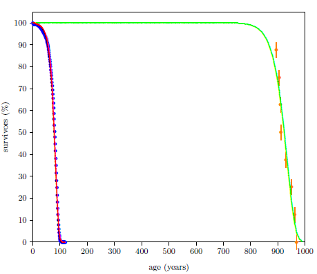There are nine pre-Flood males, from Adam to Shem, listed in Table 5.3. Shem, the last of these nine, is excluded from Figure 6.2. He lived most of his life subsequent to the Flood, and, as a result, he would have been killed by the two vitamin deficiency diseases responsible for modern human aging long before TOLA would have begun to take its toll on him. Noah displays the opposite case. He also lived several hundred years of his life after the Flood, but because he had lived nearly 700 years of his life before the Flood, he would have been killed by TOLA before his post-Flood, modern-human-aging deficiency diseases had progressed sufficiently to kill him.

The pre-Flood data presented the difficulty, for survival curve construction purposes, that the birthdates of the individuals involved were not all the same. In fact, the birthdates involved span 1,056 years. This difficulty was dealt with by assuming that dietary insufficiency of tree-of-life nutrient(s) was uniform in the pre-Flood period in question. This assumption will be valid as long as the vital tree-of-life nutrient(s) were sourced exclusively by the tree of life. In that case, exclusion from the tree of life guaranteed a uniformly zero dietary intake of the vital tree-of-life nutrient(s) to everyone pre-Flood (and, indeed, to everyone down to the present time).

Figure 6.2 shows least-squares fitted curves for both modern and ancient male survival curve datasets using the Aardsma model discussed previously:

For the ancient male survival curve, all eight datapoints are for males selected because they appear to have died of TOLA, not random death, so R was set equal to zero in the Aardsma model before the least-squares fit was carried out. The graph is somewhat remarkable. It is remarkable that the Aardsma model is able to fit the biblical life span dataset successfully. This ancient dataset exhibits a very much greater human longevity than the modern dataset, and yet the relatively simple Aardsma model is able to describe both datasets successfully. This strengthens confidence in 1) the integrity of these ancient data, 2) the utility of the Aardsma model for analyzing survival curve datasets, and especially 3) the fundamental soundness of the General Theory of Aging.

TOLA will still be active today, of course, but because it does not result in death until ages in excess of roughly 800 years have been reached (Figure 6.2), and because the two Flood-induced, congenital vitamin deficiency diseases kill everyone off long before 800 years of age have been reached (Figure 6.2), TOLA, deemed the whole cause of human aging pre-Flood, plays essentially no role in modern human aging. The present volume concerns itself with the cure of modern human aging alone. The expectation is that the cure of modern human aging will revert human aging back to TOLA, with its life spans in excess of 900 years.

The ability of the General Theory of Aging to model the more complex post-Flood life expectancy data successfully, as it has done here with the pre-Flood life expectancy data, will be shown in Chapter 19.

6.2  Conclusion

Many theories have been advanced in an effort to explain why humans age and die the way we do today. Theories multiply in science whenever none of them really works. The biblical life expectancy graph easily falsifies many existing theories, clearing the fog. When the biblical life expectancy graph is coupled with the General Theory of Aging, it points in a new direction entirely: Flood-induced congenital human diseases.

Chapter 7

The Central Hypothesis

The conclusion of the foregoing chapter is easily articulated from the vantage point offered by hindsight. Not so easy is the job which must now be embarked upon of communicating succinctly the many decades of research which were necessary to obtain this hindsight.

After years of contemplating the nature of modern human aging in light of the biblical life expectancy data, the conjecture that modern human aging must be due to a nutritional deficiency disease was born. This conjecture then rapidly developed into what I will call "the central hypothesis."

Central Hypothesis: Modern human aging is a nutritional deficiency disease resulting from dietary insufficiency of one or more vitamins, previously unknown to science, made globally deficient by the impact of Noah's Flood on earth's environment.

7.1  Deficiency Diseases

The human body is made up of trillions of microscopic cells. Each cell can be thought of as a very complex and busy city, part of a vast empire (the body). Each moment, raw materials flow into these busy cities, and, together with some waste, many finished products necessary to the overall growth, function, and maintenance of the empire flow out.

Among the raw materials flowing into these cities each moment are some which can be obtained only from outside the boundaries of the empire. For example, the human body cannot manufacture oxygen. The human body gets oxygen by breathing it in from the atmosphere. Many of these raw materials are absolutely vital to the cities—the cities cannot produce necessary finished products without them. If the supply of any one of these vital raw materials is halted for any reason (for example, lack of oxygen due to asphyxiation), then production of one or more vital finished products ceases. The prosperity of the empire then suffers and, if the lack of this vital raw material persists long enough, the empire eventually disintegrates (i.e., the body dies).

On the list of vital raw materials needed by our bodies are such things as oxygen, water, fats, amino acids, certain minerals—calcium, phosphorus, sodium, potassium, chloride, magnesium, iron, copper, iodine, and many others in minute amounts—and a curious assortment of just over a dozen organic substances we call vitamins. If for any reason the cells of the body are unable to obtain one of these vital substances, then a deficiency disease results.

The most common cause of deficiency diseases in humans is inadequate diet. The essential raw material is simply not being taken into the body. But there are other possible causes, such as a faulty digestive system resulting in inadequate absorption of an essential raw material once it has been ingested, or combination of the essential raw material after ingestion with some other chemical and subsequent elimination of the compound from the body.

Of the list of essential raw materials needed by the body, the vitamins are of particular interest in the present context. Vitamin deficiency diseases appear to be at the root of modern human aging.

7.1.1  The Example of Vitamin C

Scurvy is an example of a vitamin deficiency disease. It results from a diet deficient in vitamin C.

Before it was understood that scurvy is a deficiency disease, scurvy was a common disease of mariners. Vitamin C is abundant in fresh fruits and vegetables, so most of us get plenty of it in our normal diet each day. Vitamin C is easily subject to destruction by oxidation, however, so vitamin C levels decline in fruits and vegetables following harvest. Upon prolonged storage, vitamin C levels in fruits and vegetables become inadequate to meet human dietary requirements for this substance. The difficulty of providing mariners with fresh produce on long sea voyages inevitably resulted in many cases of scurvy.

Long before vitamin C was discovered, a number of individuals began to understand that scurvy could be prevented by a diet containing adequate fresh fruits and vegetables. Ways were sought, and eventually found, to protect the anti-scurvy property of lemons by concentrating and preserving the juice. Early in the 1800's, the British navy adopted regulations requiring daily consumption of lemon juice, bringing the scurvy plague to an end in the British navy. Eventually, this simple remedy was adopted for use on commercial vessels as well. The substitution of cheaper lime juice for the original lemon juice led eventually to the slang designation of British sailors as "limeys."

The actual anti-scurvy factor in fresh fruits and vegetables—the vitamin C molecule—was isolated, and its structure determined (Figure 7.1), only about ninety-five years ago.

Figure 7.1: Structure of the vitamin C molecule.

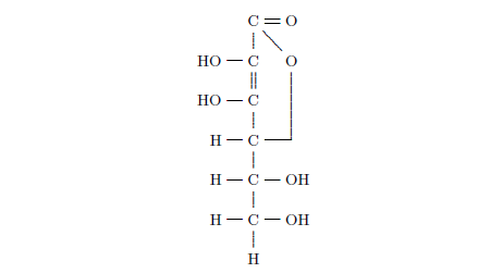Vitamin C is a relatively simple organic molecule, and it is chemically similar to the physiologically ubiquitous molecule glucose, but the human body is unable to synthesize it. This molecule is vital to human health. Without it, connective tissues between cells degenerate. This results in a complex of symptoms at the whole-organism level. Most conspicuously, blood vessels become so weak that hemorrhage results, and teeth lose their strength and become diseased.

Adult patients suffering from scurvy complain of weakness, pains in their legs, swollen and bloody gums and hemorrhages. Examination discloses petechiae, chiefly about the hair follicles of the lower extremities and sometimes brawny, tender thighs. All of these features are due to hemorrhage…

Weakness is usually the first thing complained of by persons suffering from vitamin C depletion. Fatigue, palpitation and breathlessness are also common. The patients dislike to stand or walk and often affect a rather characteristic standing position with their legs slightly flexed. The complexion is pallid and dirty looking. Gingivitis occurs, followed by loosening of the teeth, a consequence of resorption of the alveolar bones and infections about the teeth and is accompanied by a foul breath. Other signs of scurvy are hematuria, bloody diarrhea, nasal hemorrhage or hematomas about the jaw or bones of the lower extremities.^[24]

Vitamin C is needed only in minute amounts—about one ten-thousandth of our daily food intake on a dry weight-per-weight basis. This miniscule daily requirement relative to the bulk diet is characteristic of all the vitamins. In the case of vitamin D, the amount needed is roughly one five-millionth of our daily food intake. But though so little is needed, this small amount is absolutely essential. Without it, our cells lose their ability to carry out their jobs, and, eventually, a complex of whole-body symptoms—a deficiency disease—develops.

7.2  Working Hypothesis

The central hypothesis is that modern human aging is a nutritional deficiency disease resulting from dietary insufficiency of one or more previously unknown vitamins made globally deficient by the impact of Noah's Flood on earth's environment. Starting out, I didn't know that two unknown vitamins would eventually be discovered, and finding even one unknown vitamin seemed a pretty formidable task. So I restricted the working hypothesis to a single vitamin and initiated a quest to find it. For many years, before the identity of this vitamin was known, I dubbed it simply "vitamin X."

Early support for the working hypothesis that human aging is a universal, congenital deficiency disease of vitamin X was easily gleaned by comparing and contrasting modern human aging with scurvy.

7.2.1  Complex of Symptoms

Notice, first of all, that like scurvy, modern human aging exhibits itself as a complex of whole-body symptoms: skin loses its elasticity, muscles weaken and decrease in size, hair loses its color and thins out, bones become brittle, eye lenses stiffen…

These are very diverse symptoms, yet they show up together in modern human aging. One could suppose that they are all caused by independent physiological malfunctions of one sort or another, and that these independent malfunctions are all synchronized by some sort of master biological time-clock. But much simpler is the idea that these diverse symptoms are simply varied macroscopic manifestations of a single missing essential molecular component at the microscopic, cellular level—just as is the case with scurvy.

7.2.2  Particular Symptoms

Not only is there a complex of whole-body symptoms in both cases, but some of the particular symptoms of "old age" also show striking similarities to symptoms of scurvy.

Aschoff and Koch were greatly impressed with the similarity of the scorbutic [scurvy] lesions to those in senility ["old age"]. The changes in cortical bone are difficult, if not impossible to distinguish. … In both conditions the bones are notably thin and rarefied, susceptible to fracture and defective in the ability to form a callus once fracture has occurred. …

Westin interpreted the tooth lesions as similar to the atrophy of old age and said scurvy may be considered to hasten involution. In his cases the teeth showed the same resistance to caries that is seen in senility as well as the rarefaction common to advanced years.^[25]

This demonstrates that vitamin C deficiency disease can produce precisely the same sorts of abnormal changes and injury to body tissues as those which are characteristic of modern human aging. Evidently then, at least some of the specific symptoms accompanying modern human aging fall naturally within the vitamin deficiency disease category.

7.2.3  Apparent Contrast

An apparent contrast between modern human aging and scurvy is that only a small percentage of individuals in a normal population ever contract scurvy, while all individuals, if they live long enough, suffer modern human aging.

This apparent difference is easily explained by the working hypothesis. Normal diets of most individuals supply them amply with vitamin C. Only the few individuals on deficient diets ever contract scurvy. In contrast, normal diets of all individuals have become seriously deficient in vitamin X as a result of the Flood. How this came about will be explained in detail in subsequent chapters.

7.2.4  Variable Time of Onset

Another similarity between modern human aging and scurvy is that the time of onset can be varied. Prior to the Flood, men lived in excess of 900 years. After the Flood, men died of "old age" at younger and younger ages, until the present, much-diminished life span near 75 years was reached.

The time of onset of scurvy can be similarly varied:^[26]

They found that [in experiments with guinea pigs] less than 50 cc. of milk daily resulted in scurvy within thirty days, that 50 cc. delayed the onset of the disease until the seventy-fifth day and that 100–150 cc. of milk postponed evidence of scurvy for four months.

7.2.5  Why Life Spans Changed

Milk is a poor source of vitamin C. Thus all of the guinea pigs referred to in the previous quote were subject to a vitamin C deficient diet. Those getting less milk got less vitamin C. Thus the time of onset of scurvy is seen to be directly related to the daily intake level of vitamin C in the diet.

This intake-dependent time-of-onset characteristic of vitamin deficiency diseases provides an explanation of the change in human life spans following the Flood which Genesis records. It implies that human life spans changed because the availability of dietary vitamin X changed. This could happen if vitamin X was somehow produced and metered out by earth's environment to all individuals globally in a rigidly fixed intake from the time of birth on. This leads to the conjecture that life spans diminished following the Flood because vitamin X became increasingly scarce globally after the Flood so that, by 2500 B.C. (one thousand years after the Flood), vitamin X had dwindled to the seriously deficient level which characterizes it today. Subsequent chapters will demonstrate the success of this conjecture, explaining why vitamin X availability dwindled the way it did.

7.3  Conclusion

There seems to be nothing about modern human aging which is inexplicable in terms of it being a nutritional deficiency disease due to a lack of previously unknown vitamins. This category of disease seems to provide a more or less complete explanation of the facts in regard to modern human aging. This appears to be true of no other category of known diseases.

Just as scurvy results from a diet deficient in vitamin C, so modern human aging may be thought of as resulting from a diet deficient in vitamin X.

Vitamin C is called the "anti-scurvy vitamin." Following this example, vitamin X may be called "the anti-modern-human-aging vitamin" or for short, "the anti-aging vitamin."

The Flood somehow broke the natural supply of vitamin X. This caused human life spans to be reduced ultimately by a factor of more than ten relative to what they had been prior to the Flood.

Chapter 8

Properties of Vitamin X

Having adopted the working hypothesis that modern human aging results from inadequate dietary intake of vitamin X, the research goal became to identify the chemical compound—the molecule—corresponding to vitamin X. The expectation was that restoration of vitamin X to human diets would cure modern human aging just as restoration of vitamin C cures scurvy.

But identifying the compound corresponding to vitamin X was no easy task. There were nearly an infinite number of chemical compounds to choose from. It would clearly not do to try random guesses. Rather, it was necessary, like a detective, to gather every bit of information I could about vitamin X and then use these clues to try to deduce the molecular identity of vitamin X. The current chapter chronicles the beginning of this process during which two important properties of vitamin X were revealed.

8.1  The Eber–Peleg Drop

The biblical life expectancy data display a fairly uniform, natural decline from Noah to Moses. The only real irregularity in this uniform decline, allowing for normal scatter in the data points, is a sudden drop in life spans between Eber and Peleg. This irregularity is highlighted in Figure 8.1 by a line connecting the Eber and Peleg data points.

Figure 8.1: Biblical data showing life expectancy at birth for selected males. The blue line highlights a large drop in life expectancy between Eber and Peleg.

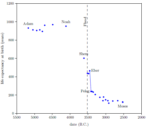This sudden drop has been used by some to argue for gaps in the Genesis chapters 5 and 11 genealogies from which many of these life expectancy data points have been taken. The argument, in this case, is that it is unlikely that life spans would have changed so dramatically in a single generation—from 464 years for Eber to just 239 years for Peleg—when they changed little in both the preceding two generations and in the following two generations.

In point of fact, there are no generations missing between Eber and Peleg. The sudden drop in life spans between Eber and Peleg is real history. That is, it really was the case that Peleg was Eber's direct, first-generation son. That this is the case will become increasingly clear in subsequent chapters.

From a modern perspective, this yields a curious result. It means that the son, Peleg, died of "old age" nearly two centuries before his father, Eber, died of "old age." Said another way, the father was yet relatively youthful when the son died of "old age."

How is such a thing possible?

Such a thing is possible if and only if vitamin X has a long biological half-life.

8.2  Biological Half-life

Biological half-life is a measure of how long a substance tends to remain in the body before it is eliminated. The biological half-life can be broken down into half-lives for individual organs, like the heart, or the kidneys. Different organs can have very different half-lives. For example, it is possible for a compound to clear from the kidneys very rapidly, but to be retained in heart muscle for a long time. It would then have a short half-life in the kidneys and a long half-life in the heart.

The overall biological half-life of a substance in the human body can be measured by giving a person a small amount of that substance and measuring the amount remaining in the body (all organs and tissues) after an elapsed time. The biological half-life is the time it takes for just one half of the original amount to be remaining.

Sodium, which we get from common table salt, sodium chloride, is used in tissues throughout the body. It has a relatively short biological half-life of just 29 days. Calcium, on the other hand, tends to get tied up in bone, and has a relatively long biological half-life of 49 years.^[27]

8.3  Biological Half-life of Vitamin X

Imagine two modern individuals, Bob and Tom, of the same age—say ten years. If neither is given supplemental intakes of vitamin X, then both will die of vitamin X deficiency disease (modern human aging) within a few decades of seventy-five years. We know this with fair certainty because billions of individuals have corroborated it since the time of Moses.

Now imagine that Bob is given supplemental intakes of synthetic vitamin X so that he gets all the vitamin X his body needs from age ten on, while Tom remains at a natural, present-day (deficient) level of vitamin X. Tom will die of modern human aging within a few decades of 75 years. But not so Bob. Bob's body will begin to heal of modern human aging and be protected against modern human aging by vitamin X, just as a person receiving an adequate diet of vitamin C will be healed of and protected against scurvy.

We see by this simple example that two individuals of the same age, living at the same time, can experience very different rates of "aging" (i.e., growing sick with vitamin X deficiency disease) depending on their respective intake rates of vitamin X.

Now imagine that Bob is given synthetic vitamin X for one year only, after which he, like Tom, receives only a natural present-day level of vitamin X. What will be the result?

If vitamin X has a biological half-life measured in days, like sodium, then the benefit to Bob of his year-long supplemental intake of vitamin X will be merely to increase his life expectancy by one or two years. Extra vitamin X can benefit Bob only while he has it in his body, and he will have it in his body for only a short while after he stops taking it if it has a short biological half-life. But if vitamin X has a relatively long biological half-life, say 49 years, like calcium, then Bob would be expected to outlive Tom by a century or more. The reason for this is that, in the case of a long biological half-life, vitamin X continues to be maintained at high levels in Bob's body long after supplemental intake has stopped.

This is what happened in the case of Eber and Peleg. Since no means of artificially synthesizing vitamin X was available back at that time, Eber and Peleg were limited to only that intake of vitamin X which the environment naturally provided. Eber was born at a time when the amount of vitamin X in the environment was much higher than it is today. Sometime during the thirty-four years between the birth of Eber and the birth of Eber's son, Peleg, the amount of vitamin X in the environment declined dramatically. There is a very good reason why the amount of vitamin X in the environment declined this way, which will be discussed in a subsequent chapter, but for now, notice merely that, as a result of this decline, the natural intake of vitamin X received by Peleg was always much less than that which his father Eber had initially received.

From Peleg's birth on, both Eber and Peleg were receiving the same, relatively low, natural intake of vitamin X from the environment. But even though they were both limited to the same natural intake rate of vitamin X from Peleg's birth on, Eber did not die of "old age" at the same time Peleg did. Eber lived on for several centuries after Peleg, his son, had died of "old age." Eber outlived his son Peleg by over two hundred years because Eber carried a higher level of vitamin X with him, in his body, long after vitamin X had declined dramatically in the natural environment.^[28] This shows that the biological half-life of vitamin X must be relatively long—measured in centuries.

The long biological half-life of vitamin X is apparent in the Genesis life span data in many other instances than just Eber and Peleg. Notice, as a single additional example, that Shem, who accompanied his father Noah on the ark, outlived not only Peleg, his great-great-grandson, but also even Terah, Peleg's great-great-grandson (and father of Abraham). Shem, born before the Flood, died of "old age" only 25 years before Abraham—born 350 years after the Flood—died of "old age."

Clearly, vitamin X has a long biological half-life.

8.4  Environmental Half-life of Vitamin X

The environmental half-life is the time it takes for just one half of an original amount of a substance to be remaining in the environment after it has been added to the environment. As with biological half-life, the environmental half-life can be broken down into various compartments. For example, the environment might be broken up into atmosphere, hydrosphere, and biosphere compartments. Each of these compartments would have its own characteristic half-life for a given compound, and these half-lives could differ substantially from one another.

Vitamin X displays two environmental half-lives, a short one and a long one, implying its presence in two environmental compartments. The long half-life compartment is apparent from the slow decline in life expectancies between Peleg and Moses (Figure 8.1). This slow decline compartment will be discussed further in subsequent chapters. The short half-life compartment is apparent from the rapidity of the drop in life expectancy between Eber and Peleg. This drop in life expectancy requires that the environmental abundance of vitamin X dropped dramatically between Eber's birth and Peleg's birth. The time between these two births was just 34 years. Thus we learn that vitamin X in the natural environment can decline dramatically in a matter of a few decades or less. This is just another way of saying that vitamin X has an environmental compartment with a relatively short half-life—on the order of a decade or less.

8.5  Conclusion

Vitamin X has an unusually long biological half-life. It has at least two environmental compartments, one with a relatively short half-life and the other with a considerably longer half-life.

Chapter 9

The Environmental Abundance of Vitamin X

At this point, I was able to begin to piece together how the environmental abundance of vitamin X changed as a result of the Flood.

9.1  The Environmental Abundance Graph

The bottom graph of Figure 9.1 shows the sudden decline in the environmental abundance of vitamin X (long vertical arrow pointing down) implied by the drop in life spans between Eber and Peleg. The slope of this environmental decline between Eber and Peleg is unknown, other than that it was steep. Keeping things simple, I have assumed that the drop was instantaneous, as the arrow depicts. The arrow is plotted midway between the births of Eber and Peleg, 3435 B.C., 85 years following the Flood.

Figure 9.1: Top: Biblical data showing life expectancy at birth for selected males. Bottom: Environmental abundance of vitamin X (the scale is arbitrary at this stage) including the sudden decrease between the births of Eber and Peleg, the Post-Peleg decline, and the drop during the lifetime of Moses.

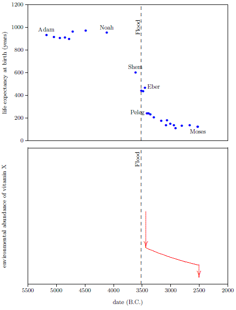The indication is that vitamin X began to decline and disappear from the environment, not at the Flood, but rather only 85 plus or minus 17 years following the Flood.

The three individuals born after the Flood but before this Eber–Peleg Drop all have rather similar life spans. Their life spans are lower than pre-Flood life spans, but this seems to be because they lived most of their lives after this drop, not because vitamin X abundance had already declined before they were born.

It thus appears that vitamin X was maintained in dietary sufficient amounts from before the Flood up until this drop. Vitamin X deficiency disease seems to have set in only some 85 years following the Flood. The reason for this will clarify in Chapter 11.

9.1.1  The Post-Peleg Decline

From Peleg to Moses, life expectancies show a relatively gentle decline (Figure 9.1, top graph). This decline in life spans implies an underlying decline in the environmental availability of vitamin X, which I have illustrated in the bottom graph of Figure 9.1.

The decline in life spans is fastest initially, so I have chosen to represent the decline by a natural exponential decay. At this point, the initial height of the exponential and how fast it should drop off are both unknown. I made initial guesses at these two parameters to get the representative exponential decline which is plotted in the bottom graph of Figure 9.1. These guesses will be mathematically refined in a subsequent chapter.

Notice that, as mentioned previously, this adds a second environmental half-life to vitamin X, one which is quite long, implying two environmental compartments.

9.1.2  The Moses Drop

Life spans appear to have rapidly dropped once again in the lifetime of Moses. In the first half of the tenth verse of Psalm 90, Moses notes that life spans had dwindled to roughly 75 years.

As for the days of our life, they contain seventy years,
Or if due to strength, eighty years,…

Moses himself lived 120 years, and his brother Aaron lived 123 years. Thus, there was another Eber–Peleg type of drop in life spans during Moses' lifetime. This drop appears to have resulted in the modern life span for humans, which has persisted now for more than 4,500 years. This final drop is indicated by the final red arrow. For simplicity, I have chosen to make this drop instantaneous once again. In real life, this final drop would almost certainly have been more gradual.

A date for this drop can be estimated as follows. Because Moses had to observe and record the drop, the latest time that persons could have begun dying of "old age" at 75 years on average is the same time Moses himself died of "old age" at 120 years. These persons would have been born when Moses was 45 years old. This places the latest date for the drop in 2482 B.C. The earliest time this drop could have happened, and Moses and Aaron still enjoy their recorded, significantly longer life spans due to the biological half-life of vitamin X, is the year following the birth of Moses. This is 2526 B.C. The best estimate, in this case, is the midpoint between earliest and latest possibilities, which is 2504 B.C.

We do not know, at present, how far the environmental abundance of vitamin X dropped at this point. This will clarify in the next chapter.

9.2  Conclusion

The environmental abundance of vitamin X breaks naturally into four distinct time periods. These are depicted in the bottom graph of Figure 9.2.

Figure 9.2: Top: Biblical data showing life expectancy at birth for selected males. Bottom: Environmental abundance of vitamin X showing four distinct time periods.

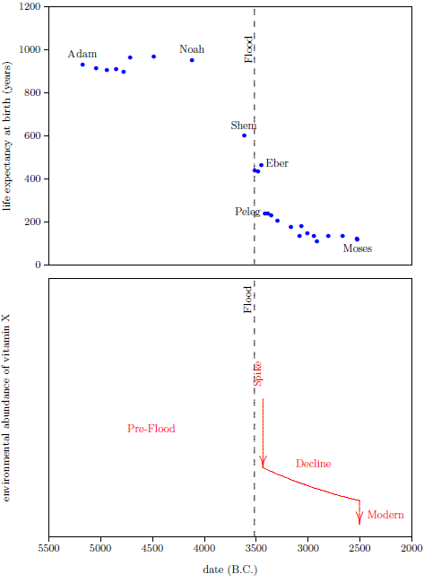The first is the "Pre-Flood" time period. This is a steady state region, in which the environmental availability of vitamin X, while dietarily sufficient, is unknown but assumed to have been constant and relatively high. This region ended with the coming of the Flood.

The second time period, initiated by the Flood, ended with a sharp reduction in environmental availability of vitamin X sometime between the births of Eber and Peleg. This might be called the "Pause," as in "the pause before the storm," highlighting the fact that vitamin X deficiency disease had not yet begun, but I have labeled it "Spike" for reasons which will soon become apparent.

The third is the "Decline" time period. Environmental availability of vitamin X, which was already seriously deficient at the beginning of this time period, slowly declined, becoming ever more seriously deficient during this time period.

The fourth is the "Modern" time period. It was ushered in roughly 2504 B.C. by a final rapid drop in life spans to the modern value near 75 years, which took place during the lifetime of Moses.

Chapter 10

The Natural Synthesis and Distribution of Vitamin X

It was at this point possible to advance reasonable answers to three key questions.

1. How was vitamin X distributed by nature?
2. How was vitamin X synthesized by nature?
3. How did vitamin X enter the human diet?

10.1  How Was Vitamin X Distributed by
Nature?

The biblical life span data seem to imply that, while longevity varied widely in different periods of history, it was globally uniform at a given point in time. The biblical longevity data do not encompass a global population, of course, but they do extend over a large enough geographical area in the Middle East—including at least portions of modern Iraq, Turkey, Israel, and Egypt—to make global uniformity seem likely.

Is there any way of explaining a point-in-time geographical uniformity of vitamin X given its large temporal variations?

Yes. The atmosphere is present globally, and it mixes rapidly relative to human life spans—just a year or two from pole to pole. If vitamin X were distributed by the atmosphere, then its consequences for longevity would be globally uniform at any point in time.

The atmosphere is made up of gases. The mixture of gases comprising the atmosphere is called air. Nitrogen and oxygen are the main gases in air, but there are many gases present in minor amounts as well. For example, nearly one percent of air is the gas called argon. Well-known gases in air include ozone, carbon dioxide, and methane. Dozens more, not so well known, like carbon disulfide and nitrogen dioxide, might easily be mentioned. All of the gases in air, other than nitrogen and oxygen, are called trace gases. Point-in-time global uniformity would be explained if vitamin X were a trace gas or were somehow involved with a trace gas.

The idea that vitamin X is somehow involved with a trace gas provides an explanation of the Decline time period of the vitamin X environmental abundance graph. In the previous chapter (Figure 9.2), the Decline was shown lasting roughly 900 years. The Flood seems to have broken the fundamental source of vitamin X, but vitamin X did not drop immediately to zero following the Flood. Rather, it waited some 85 years, dropped down suddenly, and then slowly declined for 900 years. Involvement of a trace gas provides an explanation of this prolonged decline. Specifically, there is a component of earth's global environmental system which has this characteristic timescale. One thousand years is the order-of-magnitude timescale for the turnover of earth's oceans. Deep ocean water takes roughly a thousand years to move from the bottom of the ocean to the surface. A change lasting 900 years would be expected if the oceans acted as a reservoir for the conjectured atmospheric trace gas. Gases have a water solubility. Gas molecules, present in earth's oceans, are effectively cut off from the atmosphere. They can get out of the ocean and into the atmosphere only by diffusion through the ocean–atmosphere interface at the surface of the ocean. Gas molecules down deep in the ocean will be stuck in the ocean for hundreds of years waiting for the water in which they are trapped to move slowly up to the surface, where they can vent to the atmosphere via diffusion through the surface. The 900 years of the Decline time period can be readily explained as the time it took for the trace gas involved with vitamin X to empty out of the oceans into the atmosphere.

Said succinctly, though the Flood broke (i.e., shut down) the primary source of some atmospheric trace gas, the oceans continued to act as a source of this gas to the atmosphere until their supply had been exhausted roughly 900 years later. With the trace gas exhausted, the environmental concentration of vitamin X went to zero and could go no lower, explaining why human life spans have been constant at roughly 75 years for thousands of years ever since.

All of this argues forcefully for the idea that vitamin X was distributed globally via the atmosphere, either as a trace gas or as some atmospheric product of a trace gas.

Notice that this also explains why the environmental abundance of vitamin X has a fast environmental half-life compartment and a slow environmental half-life compartment. The fast compartment is the atmosphere, and the slow compartment is the oceans.

10.2  How Was Vitamin X Synthesized by
Nature?

The idea that vitamin X is a trace gas, while possible, is less attractive than the idea that vitamin X is a product of a trace gas. The reason for this has to do with the nature of the thirteen traditional vitamins and the nature of the atmospheric chemistry of trace gases.

To begin with, of the thirteen traditional vitamins, none are gases. Vitamin-likeness argues against vitamin X being a gas.

The atmosphere contains a lot of oxygen. Atmospheric chemistry tends either to break a trace gas down into smaller fragments, or to add a few oxygen atoms to a trace gas. Breaking a trace gas down into smaller fragments will yield yet lower molecular weight products, which will tend to be gases. Thus, vitamin-likeness favors the oxygen-addition process over the fragmentation process. Atmospheric chemistry argues for vitamin X being a small molecule. Atmospheric trace gases tend to be small molecules. Large molecules are too massive to have sufficient vapor pressure to be present in the gas phase. There is no sharp mass cutoff for presence of a compound in the atmosphere, but a molecular weight of 250 g/mole seems to be a reasonable dividing line above which few molecular substances are likely to be found in significant abundance in the atmosphere.

This small-molecule dividing line places vitamin X in the water-soluble vitamin category. Of the thirteen traditional vitamins, nine are water-soluble and four are fat-soluble. None of the fat-soluble vitamins has a molecular weight below 250 g/mole, while five of the water-soluble vitamins have molecular weights below this cutoff. Thus, vitamin-likeness argues for vitamin X to be a small, water-soluble molecule.

Does the atmospheric chemistry, oxygen-addition process tend to produce water-soluble products?

Yes. Oxidation of trace gases tends to yield small acids as stable end products. Small acids are notoriously water soluble.

Are any of the small water-soluble vitamins acids?

Yes. In fact, of the five water-soluble vitamins having molecular weights below 250 g/mole, four are acids.

Thus, the idea that vitamin X is a small acid, an oxidation product of an atmospheric trace gas, is very attractive.

10.3  How Did Vitamin X Enter the Human Diet?

This idea immediately answers the third question. Because small acids are soluble in water, acids produced in the atmosphere are rapidly washed out of the atmosphere by rain once they have been formed. This means that they are naturally present in rainwater, in freshwater ponds and lakes, and in rivers. Clearly, vitamin X would have entered human diets in antiquity via the water that humans drank.

10.4  The MSA Example

Methanesulfonic acid (MSA) is an example of a small organic acid which is produced in the atmosphere by oxidation of a trace gas.^[29] The trace gas in this instance is the extensively studied dimethyl sulfide (DMS).

DMS is naturally produced in ocean surface waters from di-methylsulfoniopropionate (DMSP), which is a metabolite of some marine algae. In the atmosphere, DMS reacts with the hydroxyl radical (OH•) or the nitrate radical (NO₃•) resulting in oxidation to a variety of products, including MSA.

MSA concentrations in glacier ice are generally around 10 micrograms per liter. Thus, use of rainwater for drinking today (not recommended due to ubiquitous pollutants in modern air) would naturally supply human diets with 20 micrograms or more of MSA per day. This is not to suggest that MSA is desirable in human diets today, but rather to show that nature is capable of producing and supplying to the human diet compounds in vitamin-like quantities via an atmospheric trace gas.

10.5  Conclusion

The idea that vitamin X is a small acid, an oxidation product of an atmospheric trace gas, is compelling. It provides satisfying explanations of the natural synthesis, distribution, and dietary presence of vitamin X.

Chapter 11

What the Flood Broke

Having deduced that vitamin X seemed likely to be an oxidation product of an atmospheric trace gas, the next strategic goal was to try to identify the trace gas, as an aid to identifying vitamin X. There were, unfortunately, still way too many trace gases (giving rise to a plethora of oxidation products) to make random guessing a feasible research strategy. It was necessary to make use of every clue once again. But this time, it was knowledge of the nature of the Flood, not the properties of the trace gas, which resulted in the vital breakthrough.

11.1  The Nature of the Flood

The vitamin X precursor trace gas was being supplied to the atmosphere pre-Flood in much greater abundance than it is at present. The Flood somehow broke the supply to the atmosphere of this precursor gas.

How might the Flood have broken the supply of an atmospheric trace gas? The answer to this question seemed likely to provide the all-important clue to learning the identity of vitamin X. Thus it appeared that finding the cure for modern human aging required "only" a thoroughgoing understanding of the true nature of Noah's Flood. Fortunately, I had such an understanding.

Reword that. In actual fact, good fortune had little to do with it. I had spent decades of my life uncovering the truth regarding Noah's Flood. I had found that mainstream academia is seriously mistaken about the Flood. Modern academicians seem to regard it as essentially mythological, if they bother to think about it at all. And I had found that individuals holding out against the view that the Flood was a myth (usually for theological reasons) were generally seriously mistaken in their understanding of the true nature of the Flood. In consequence, none were very well positioned to be of much help in regard to the question of how the Flood might have broken the supply of an atmospheric trace gas. It was, therefore, necessary to solve the mystery of the true nature of Noah's Flood before the mystery of modern human aging could hope to be solved.

The important thing to know about the Flood in the present context is that it was hemispherical in extent. It resulted from the waters of the southern hemisphere flowing up into the northern hemisphere and heaping up to great depth there for some months. Why this happened—the geophysics behind it—is explained in detail in the book, "Noah's Flood Happened 3520 B.C.,"^[30] so I will not go into detail here. The important thing to notice at present is only this: heaping the planet's oceans up in the northern hemisphere will expose the sea floor in the southern hemisphere. In fact, the sea floor in the high southern latitudes surrounding Antarctica was entirely uncovered for at least 110 days during the Flood.

11.2  The Nature of Sea Floors

Sea floors are hidden from our eyes. As a result, they are not items of common knowledge. The important thing to know about them at present is that they are covered with sediments. The average depth of the sediments covering the floors of the world's oceans exceeds a quarter of a mile.

Sea floor sediments are cut off from atmospheric oxygen. In consequence, they are anaerobic. Anaerobic microorganisms in organic-rich sediments produce organic gases as byproducts within those sediments. Methane is a major, well known byproduct gas of anaerobic digestion. Other anaerobic byproduct gases include, for example, carbon dioxide, hydrogen, nitrogen, and hydrogen sulfide.

11.3  The Source of the Precursor

I conjectured that the source of the atmospheric trace gas which is the precursor to vitamin X was anaerobic digestion of organic detritus within the sea floor sediments of the southern oceans. Steady state diffusion of molecules of this trace gas from the sediments to the overlying ocean water is what the Flood broke. The Flood broke this steady state diffusion by removing the great depth of water which normally covers the sediments. This reduced the pressure these sediments are normally under by hundreds of atmospheres. (Each ten meters of water depth adds another atmosphere of pressure, and the average depth of the oceans is 3800 meters.) The inevitable result was rapid release (outgassing) to the atmosphere of the anaerobic byproduct gases contained within these sediments.

11.4  Conclusion

The Flood broke the steady state diffusion of anaerobic gases from the sediments to the bottom waters of the southern oceans by emptying southern sediments of their gases during the year of the Flood.

This produced a spike of vitamin X precursor gas in the atmosphere (which is where the "Spike" label comes from). The Flood released thousands of years' worth of vitamin X precursor gas from the sediments into the atmosphere all in one year. The result was decades of abnormally high vitamin X production in the atmosphere during the Spike.

When the atmosphere had finally managed to cleanse itself of vitamin X precursor (and the load of other sea floor gases), only precursor diffusing out of the water of the oceans remained to supply vitamin X. This explains the Decline.

When the oceans' supply of precursor ran out, life spans dropped to near 75 years, initiating the Modern time period.

The sediments of the southern oceans were emptied of their store of precursor gas by the Flood. This vital source of precursor has so far not recovered in five and a half thousand years.

Chapter 12

Vitamin X Candidates

It seemed clear that the vitamin X precursor gas had been predominantly produced in the sediments of the southern oceans.

The sediments of the northern oceans would not have been emptied of their gases by the Flood since they were never depressurized. If the source of vitamin X precursor gas were evenly distributed around the globe before the Flood, then vitamin X abundance should have been cut only roughly in half following the Flood. But we have seen that vitamin X abundance appears ultimately to have dropped to zero. Furthermore, if vitamin X precursor gas production had been spread out over the sea floor of the entire planet, then the supply of precursor gas should have shown some recovery over the past five and a half thousand years, with a correspondingly noticeable recovery in life spans, due to a natural recovery of precursor gas within those particular sediments which had been only slightly depressurized by the Flood. But no such recovery in life spans has been seen. Thus, available data seemed to favor the idea that nearly the entire source of precursor was destroyed by the Flood.

This focused attention on the southern sea floor. What was so special about it? Why did depressurization of just the southern sea floor destroy nearly the entire source of vitamin X precursor gas?

Modern ocean properties suggested answers to these questions. Phosphate and nitrate are broadly important for biological productivity. Lack of one or the other of these nutrients often limits biological productivity within the global marine environment. But the surface waters of the oceans surrounding Antarctica are especially rich in phosphate and nitrate. Figure 12.1 shows a world map of annual mean sea-surface phosphate.^[31] Figure 12.2 shows the same thing for nitrate.^[32] The existence of both of these nutrients together in high concentrations in the ocean surface waters surrounding Antarctica more or less guaranteed accumulation of organic-rich sediments on the sea floor surrounding Antarctica.^[33] Indeed, it seemed appropriate (if a trifle prosaic) to regard the sea floor surrounding Antarctica as the planet's septic tank.

Figure 12.1: 2009 annual mean phosphate at the surface.

Figure 12.2: 2009 annual mean nitrate at the surface.

12.1  A Phosphorus Trace Gas

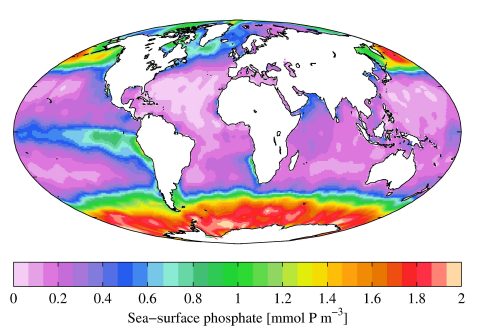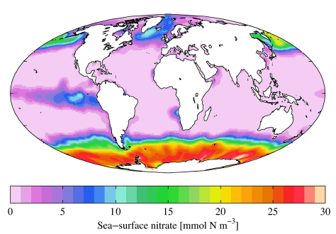The concentration of phosphorus in surface waters surrounding Antarctica makes the planet's septic tank a rich depository of phosphorus-laden biomolecules. The presence of this rich accumulation of biophosphorus instigated the hypothesis that the vitamin X precursor was a phosphorus gas byproduct of anaerobic digestion within pre-Flood sea floor sediments.

This hypothesis encountered an immediate difficulty. Phosphorus is well-known not to have any significant trace gases. In fact, phosphorus contrasts with other elemental environmental cycles in not having any significant atmospheric component. For example, the nitrogen cycle has an obvious atmospheric component in the form of N₂ gas. Similarly, the oxygen cycle has an obvious atmospheric component in the form of O₂ gas. The sulfur cycle has the already-mentioned DMS as a significant atmospheric component. DMS moves 15–25 million metric tons of sulfur from the oceans into the atmosphere each year.^[34] The environmental iodine cycle has methyl iodide (MeI) as an atmospheric component. The environmental carbon cycle has carbon dioxide (CO₂) as an atmospheric component. …   But there is no atmospheric component in the case of phosphorus.

I conjectured that this difficulty was apparent only. If one supposes that the phosphorus cycle is presently operating in steady state—that it has been behaving for time out of mind just as it is observed to be behaving at present—then the presently observed lack of an atmospheric phosphorus component leads immediately to the conclusion that it is the nature of the phosphorus cycle to be without any significant atmospheric component. But as soon as one knows the truth about the Flood, one knows better than to suppose that the phosphorus cycle is presently operating in steady state. I conjectured that phosphorus normally has an atmospheric component, in analogy with other elemental biogeochemical cycles, but that the present time is not normal, at least as far as phosphorus is concerned. I conjectured that the atmospheric component of the environmental phosphorus cycle is the fundamental thing which the Flood broke. And I conjectured that it was this breakage which resulted in the loss of human longevity following the Flood—that loss of the atmospheric component of the phosphorus cycle (i.e., loss of this phosphorus trace gas) meant loss of the vitamin X precursor, resulting in loss of vitamin X itself. The fact that the environmental phosphorus cycle is not represented by any atmospheric component today does not mean that this was the case before the Flood. Phosphorus gases do exist and are well known in the chemistry laboratory and in industry.

Phosphine (PH₃) is the simplest gas containing phosphorus. It is a possible pre-Flood phosphorus trace gas candidate, but it is not a possible vitamin X precursor candidate. Vitamins are organic compounds (i.e., they contain one or more carbon atoms). Phosphine is not organic. Atmospheric chemistry can add oxygen atoms to a precursor gas; it cannot add carbon atoms. Thus, the precursor gas must start out as an organic compound.

Simple organic trace gases of the elements often result from addition of one or more methyl groups (CH₃) to the element. An example is methyl iodide (MeI), already mentioned. MeI is sourced to the atmosphere from the oceans. The oceans also source methyl chloride (MeCl) and methyl bromide (MeBr) to the atmosphere. Dimethyl sulfide (DMS or Me-S-Me) is an example of a trace gas containing two methyl groups. It, too, is sourced to the atmosphere from the oceans.

I was looking for a simple organophosphorus trace gas sourced to the atmosphere from the oceans. Methylated phosphorus gases seemed to be the obvious choice.

12.1.1  Methylated Phosphorus Gases

The biological pathway by which methylated phosphorus gases might arise in anaerobic sedimentary environments had yet to be demonstrated by science. It seemed, however, that discovery of such a pathway was imminent.

There are strong indications that phosphine and other reduced phosphorus compounds can be produced biogenically.^[35]

Two different modes of production of methylated phosphorus gases could be imagined: 1. biomethylation of phosphorus, and 2. catabolism of phosphonates.

Biomethylation in general is well studied and reasonably well understood.

Biomethylation is the process whereby living organisms produce a direct linkage of a methyl group to a metal or a metalloid, thus forming metal-carbon bonds. Methylation has been extensively studied and biomethylation activity has been found in the soil, but mainly occurs in sediments in e.g. estuaries, harbors, rivers, lakes and oceans. … Anaerobic bacteria are believed to be the main agents of biomethylation in sediments and other anoxic environments.^[36]

From a purely utilitarian perspective, however, the second possibility, catabolism of phosphonates, seemed to me to be somewhat more attractive than biomethylation.

Phosphonates are chemical compounds having a carbon atom (C) bonded to a phosphorus atom (P). Catabolism is the process by which living organisms break down complex molecules into simpler molecules during metabolism.

In the pre-Flood anaerobic, organic-rich, phosphate-rich marine sedimentary environment surrounding Antarctica, microbes might naturally be expected to have been present which possessed an ability to "mine" phosphonates for their oxygen atoms while discarding the less readily catabolized C-P moieties as methylphosphine (MeP) "tailings," since both carbon and phosphorus would be abundantly available in more easily catabolized forms. The great versatility of microbial life made it seem likely that some anaerobic microbe having ability to exploit this environment in this way should exist.

From chemistry, it is known that phosphorus can add one, two, or three methyl groups, giving methylphosphine (MeP), dimethylphosphine (DMeP), and trimethylphosphine (TMeP), respectively. Of these three, TMeP is the least interesting for the present purpose. It has a boiling point of 38–40^°C, which means that, in the laboratory, it is a liquid rather than a gas. TMeP vapor oxidizes in the atmosphere to trimethylphosphine oxide (TMePO). TMePO is not easily oxidized a second time, and it is a severely hygroscopic solid, which means that it will be rapidly washed out of the atmosphere. If vitamin X is a small acid, as expected, then TMePO, which is not an acid, is not vitamin X.

Both DMeP and MeP are true laboratory gases. Both yield small acids upon oxidation in the atmosphere.

DMeP oxidizes first to dimethylphosphine oxide (DMePO). This is a liquid with a boiling point of 220^°C. Like TMePO, this is likely to wash out of the atmosphere. However, it can oxidize further to dimethylphosphinic acid (DMePiA).

The final methylated phosphorus compound and potential vitamin X precursor, the gas MeP, oxidizes first to methylphosphine oxide (MePO). MePO is not very stable. It easily oxidizes a second time to methylphosphinic acid (MePiA). This small acid is hygroscopic; it will wash out of the atmosphere. However, it is readily susceptible to further oxidation, either in the gas phase or in aqueous solution, yielding methylphosphonic acid (MePA) as the stable final product.

Thus, two precursor gases (DMeP and MeP) and three vitamin X candidates (DMePiA, MePiA, and MePA) resulted from methylated phosphorus.

Examining the Methylated Phosphorus Vitamin X Candidates

DMePiA is the least interesting of these three vitamin X candidates. It is a phosphinate. Phosphinates have either one carbon atom and one hydrogen atom or two carbon atoms bonded to the phosphorus atom. Phosphinates appear to possess severely limited natural biological utility.

Phosphinothricin (PT), a non-proteinogenic amino acid found in a number of peptide antibiotics, is the only known phosphinic acid natural product.^[37]

In sharp contrast, phosphonates (which have just one carbon atom and no hydrogen atom bonded to the phosphorus atom, as with MePA) appear to have ubiquitous biological utility. Phosphonates have an especially large abundance in the marine environment^[38] and in some marine organisms.

… eggs of the freshwater snail Helisoma contain 95% of their phosphorus in the form of 2-aminoethylphosphonate-modified phosphonoglycans, whereas the sea amenaea Tealia possesses up to 50% of its phosphorus in a variety of phosphonolipids, phosphonoglycans and phosphonoglycoproteins. Other organisms, such as the protist Tetrahymena, have lower overall levels of phosphonate, but still synthesize as much as 30% of their membrane lipids in the form of phosphonolipids. The prevalence of C-P compounds in nature is perhaps best exemplified by the recent discovery that as much as 20-30% of the available phosphorus in the world's oceans is comprised of phosphonic acids.^[39]

The ubiquitous biological utility of the phosphonates within the marine environment implies that a catabolic route to vitamin X precursor formation exists for MeP alone. MeP has only one carbon atom bonded to the phosphorous atom, while DMeP has two carbon atoms bonded to the phosphorous atom. Thus, formation of MeP may reasonably be expected as a byproduct of catabolism of ubiquitous phosphonate substrate in an anaerobic marine environment, but the catabolic production of DMeP would require abundant phosphinate substrate, which, as we have just seen, does not appear to exist in nature.

Thus, the lack of a catabolic route to formation of DMeP as vitamin X precursor rendered DMePiA of low interest.

This left MeP as the sole interesting vitamin X precuser gas, with both MePiA and MePA as interesting vitamin X candidates arising from methylated phosphorus (Figure 12.3).

Figure 12.3: Atmospheric precursor gas methylphosphine (MeP) and the two vitamin X candidates it presents, methylphosphinic acid (MePiA) and methylphosphonic acid (MePA).

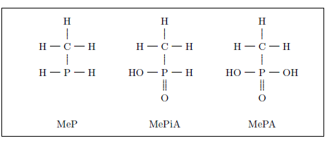MePA was of great interest as a potential vitamin X candidate. It is the simplest member of the phosphonate class of compounds. Phosphonates as a class are biologically versatile compounds with "potent bioactive properties."^[40] MePA thus appeared appropriately positioned to fill the role of a vitamin having anti-aging potency.

But, in a curious and unexpected fashion, interest in the MePiA candidacy surpassed even the great interest warranted by the MePA candidacy.

It might be thought that the evident lack of biological utility of the phosphinates would play against the MePiA vitamin X candidacy since methylphosphinic acid is a phosphinate. How, for example, could MePiA participate in the sort of biomolecule building activity exemplified by some of the traditional vitamins (e.g., in their use as organic cofactors and prosthetic groups of larger enzymes) given the near-zero biological utility of the phosphinates? The ubiquitous biological utility of the phosphonates opens the door wide for the MePA vitamin X candidacy. Conversely, the near-zero biological utility of the phosphinates seems to all but close the door on the possibility that MePiA might be a vitamin.

However, curiously, the door does not close on the MePiA candidacy if the biological utility of MePiA is merely for it to act as an antioxidant (i.e., a substance which "soaks up" reactive oxygen species [ROS]). In the process of soaking up ROS, MePiA is converted to MePA. Thus, while MePiA, as a phosphinate, might not be expected to participate in the sort of biomolecule building which is characteristic of some of the traditional vitamins, it might still function in a vitamin-like antioxidant capacity, and, in the process, yield a phosphonate product, MePA, which might then very well be expected to participate in biomolecule building and enzymatic processes similar to other vitamins.

Once this much had been understood, MePiA suddenly appeared to be a vital missing piece of a long-standing theory of aging proposed by Denham Harman, specifically, his free radical theory of aging in its final, mitochondrial form.^[41] Harman postulated that aging is caused by accumulation of biomolecular damage due to free radicals (often called ROS in biological contexts) generated during normal cell metabolism. A strategy to limit damage due to ROS is to make antioxidants (i.e., easily oxidized compounds) available to the cells. The antioxidants will then be on hand to soak up the ROS and thereby keep them from reacting destructively with cellular biomolecules.

Harman found that the average life span of mice could be increased by large daily intakes of select antioxidants. This corroborated the basic idea of free-radical damage as a cause of aging. However, somewhat surprisingly, Harman found that maximum life spans of mice could not be increased in this way.

This led Harman to postulate that the mitochondria (the locus of highest ROS concentration) were the main site of life-limiting free-radical damage and that possibly the mitochondria, which have a double membrane prohibiting entry of most compounds, were inaccessible to his antioxidants.

Harman's theory invokes the use of antioxidants as a cure for aging. Several of the vitamins are antioxidants. More to the point, vitamin-X-candidate MePiA is an antioxidant. The postulate presented itself that MePiA is the missing antioxidant needed to complete Harman's theory. I will call the theory which results from this postulate the Vitamin MePiA Theory of Aging.

Vitamin MePiA Theory of Aging: MePiA is the antioxidant vitamin needed to complete Harman's free-radical theory of aging. MePiA has special access to the mitochondria. Dietary intake of MePiA regulates the rate of ROS damage to mitochondria, which regulates the rate of modern human aging.

This Vitamin MePiA Theory of Aging is fortified by its immediate ability to explain the previously discussed observation, from the biblical life expectancy data, that vitamin X must have an unusually long biological half-life—measured in centuries. This observation is otherwise difficult to explain. No traditional vitamin has such a long half-life in the body. The biological half-lives of the water-soluble vitamins are notoriously short. Vitamin C has a biological half-life of 10 to 20 days, for example. And even the longer-retained fat-soluble vitamins still tend to have biological half-lives measured in just days or weeks. Vitamin E appears to be exceptional, with a biological half-life of a few years, but no traditional vitamin comes close to a biological half-life of a century.

The idea that MePiA has special access to mitochondria implies that specialized transport proteins exist to take MePiA molecules through the double membrane into the mitochondria, concentrating and keeping MePiA there. This implies genetic support of the protective role played by MePiA in the mitochondria. And this invokes the possibility of genetically programmed enzymes to recycle/reactivate MePiA molecules following their reaction with free radicals in the mitochondria. Genetically programmed sequestering and/or recycling of MePiA in the mitochondria is perhaps the only biological conservation mechanism capable of explaining the extremely long biological half-life of vitamin X.

12.2  Conclusion

MeP appears to be the vitamin X precursor gas, and MePiA appears to be the dominant candidate for vitamin X with MePA a secondary candidate.

Chapter 13

Choosing Vitamin X

Once the Vitamin MePiA Theory of Aging developed in the previous chapter had clarified, a longevity experiment with laboratory mice was launched to test the theory.

MePiA, according to the theory, acts as an antioxidant in the body to mitigate damage due to free radicals, in accordance with Harman's mitochondrial free-radical theory of aging.^[42] The theory says that dietary intake of MePiA controls the rate of modern human aging. This makes cellular/mitochondrial presence of MePiA to be the key to observing life lengthening in mice.

Small exploratory experiments on mice treated with MePA alone had shown no life lengthening. This implied that mice lacked any enzyme capable of converting dietary MePA to MePiA, which meant that direct administration of MePiA would be necessary to observe life lengthening.

MePiA is oxidized to MePA by free radicals of the reactive oxygen species (ROS) group. This makes MePA available in vivo where it may then operate in a typical vitamin capacity in a variety of biochemical reactions. To test for effects of MePiA alone, it is therefore necessary to treat the control group with MePA alone to counteract its inevitable accompaniment of MePiA.

To test the Vitamin MePiA Theory of Aging, an MePA-vs-MePiA mouse experiment was launched. The working hypothesis at the launching of the MePA-vs-MePiA mouse experiment was that dietary intake of MePiA was essential to obtain life lengthening. The expectation was that only the mice receiving MePiA would show life lengthening—that MePiA was vitamin X.

The best concentrations of MePiA and MePA to use in this experiment were unknown. Mice are not humans, so it was not clear that concentrations suitable to humans would be efficacious with mice. Harman had used very large concentrations of the antioxidants he had tested with mice relative to normal vitamin amounts.^[43]

I decided to use the largest practical concentrations I could afford. Water-soluble vitamins are characteristically low in toxicity, and no signs of toxicity due to either vitamin had been seen in earlier experiments. My aim was to guarantee that any life-lengthening effect intrinsic to either vitamin would not be missed.

I ended up using 0.1 grams (100,000 micrograms) of MePA per liter of drinking water and 0.1 grams of MePiA per liter of drinking water. Because these compounds are acids, these concentrations result in a low (acidic) pH. To avoid potential palatability and dentition issues with the mice, both solutions were neutralized using sodium hydroxide. Thus, the compounds tested were disodium methylphosphonate and sodium methylphosphinate.

Life span experiments with mice take several years to run to completion. It has previously been described how early results from this experiment seemed contrary to the Vitamin MePiA Theory of Aging, leaving MePA as the sole anti-aging vitamin, and how it took two years for this mistaken impression to be corrected.^[44] The present chapter summarizes the final results of this experiment. It shows that the mice receiving MePiA did experience life lengthening, corroborating the Vitamin MePiA Theory of Aging.

13.1  The Data

Figure 13.1 shows the final graph of the MePA-vs-MePiA dataset. Each treatment group began with 4 cages containing 9 mice each, all of the same age. One cage was removed from the MePiA dataset due to a treatment-unrelated, juvenile die-off event.^[45] The graph shows that the percentage of survivors in the group of MePiA-treated mice surpassed the percentage of survivors in the group of MePA-treated mice from about 110 weeks of age onward. More importantly from the perspective of aging research,^[46] the maximum life span for the MePiA mice was significantly greater than the maximum life span for the MePA mice. Taken at face value, this graph shows life lengthening of the MePiA mice relative to the MePA mice.

Figure 13.1: Survival curve datasets for the MePA-vs-MePiA-treated ICR female weanling mice experiment. The blue group was treated with 0.1g MePA per liter of drinking water, and the red group was treated with 0.1g MePiA per liter of drinking water. Treatment commenced at 24.7 weeks of age and ended at 109.6 weeks of age. Treatment was resumed at 161.9 weeks in an effort to keep the final surviving mouse alive as long as possible.

13.2  Is it Real?

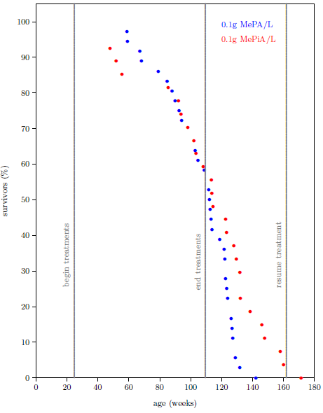Extension of maximum life span is extremely difficult to achieve. On the global research scene, only a very few interventions, such as calorie restricted diets, have succeeded in demonstrating an extension of maximum life span in mice. Though my research with various vitamin X candidate substances had attempted to demonstrate life lengthening for multiple decades with many hundreds of experimental animals—gerbils, fruit flies, vinegar worms, mice, and rats—this was the first time any evidence of increased maximum life span had been seen in my work.

Was this observed life lengthening real, or was it just a statistical fluctuation? To answer this question, I added to the graph in various shades of green all of the data my lab had ever produced using batches of same-age, weanling, female, ICR mice. There had been three additional batches in this category, spanning nearly two decades. These batches had been subjected to a variety of treatments back in their day, intended to induce life lengthening—all of which had uniformly failed in this purpose. Figure 13.2 shows that, for roughly 50% or fewer survivors, the survival curve for the MePA mice (dark blue dots) is similar to the older three batches of ICR mice, while the survival curve of the MePiA mice (red dots) clearly differs from the older three batches. MePiA treatment does indeed appear to have extended the maximum life span for these mice. It appeared that MePiA had been confirmed as vitamin X.

Figure 13.2: Survival curve datasets for the MePA-vs-MePiA-treated ICR female weanling mice experiment. Three additional batches of the same type of mice raised in the same lab in previous years but never treated with either MePA or MePiA are plotted in various shades of green.

13.3  Discussion

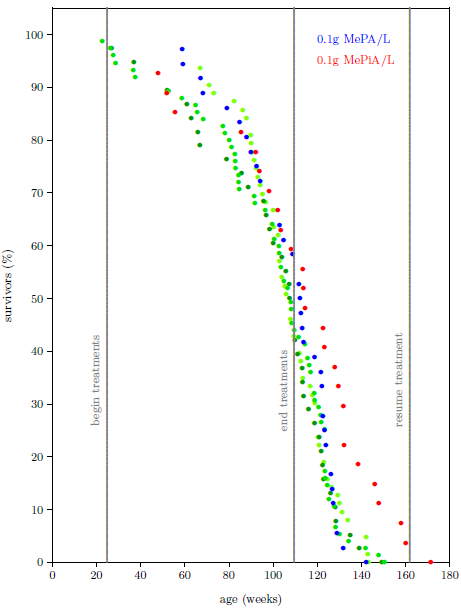The Vitamin MePiA Theory of Aging provides the following explanation of Figure 13.2.

For the first six months of their lives, before treatment with MePA or MePiA began, all mice aged at a normal rate due to mitochondrial degradation occasioned by free radicals generated within their mitochondria. Following initiation of treatments, MePA mice continued to age at a normal rate, MePA being resistant to oxidation and hence offering no protection against free radicals. Meanwhile, aging in MePiA mice was slowed due to the presence in their mitochondria of easily oxidized MePiA.

The mitochondria of MePiA mice suffered progressively less damage than the mitochondria of MePA mice throughout the treatment phase and, given the long biological half-life of MePiA in humans, probably after treatment had ceased. As a result, the MePiA-treated mitochondria were able to sustain post-treatment damage for a longer time than the MePA-treated mitochondria before critical damage levels, resulting in death, were reached. This evidenced as lengthened life spans of the MePiA mice relative to the MePA mice.

13.4  Check

A second experiment was undertaken at this point to check and improve upon the life-lengthening result of the first experiment.

The treated group of mice was once again given 0.1 grams of MePiA per liter of drinking water, but this time the control group was given just 0.8 milligrams (or 0.0008 grams) of MePA per liter of drinking water. This concentration of MePA matched the concentration of MePA present in the 0.1 grams of MePiA per liter of drinking water treatment due to natural oxidation of MePiA to MePA during MePiA synthesis. The objective was to isolate the life-lengthening effect of MePiA.

To improve the statistics, 52 mice per group (13 cages with 4 mice per cage) were used rather than the 36 mice per group (4 cages with 9 mice per cage) used with the first experiment. To increase life lengthening, the age at which treatment was begun was reduced and the length of treatment was increased with the second experiment. The expectation was that the MePiA mice would show even more pronounced life lengthening relative to the MePA control group than had been observed with the first experiment. Figure 13.3 shows that the actual outcome was more or less opposite to this expectation. The MePA mice did overall better than the MePiA mice.

Figure 13.3: Survival curve datasets for the second ICR female weanling mice experiment. The treatments shown commenced at 5.4 weeks of age and ended at 114.7 weeks of age. Three additional batches of the same type of mice raised in the same lab in previous years but never treated with either MePA or MePiA are plotted in various shades of green as previously to provide a visual reference for gauging life lengthening due to the treatments.

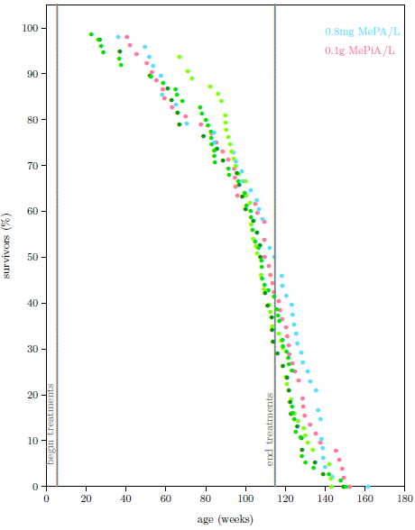In science, an experiment which comes out opposite to expectation is a most valuable experiment. It forcefully falsifies mistaken ideas, clearing the way to a better understanding. This second mice experiment corrected several mistaken ideas.

13.4.1  Correction 1: Megadose MePiA is Toxic

The first mistaken idea was that very high concentrations—megadose concentrations—of MePiA were not toxic.

The MSA example, discussed previously, suggested that the natural concentrations of this vitamin pre-Flood would have been on the order of 10 micrograms per liter of drinking water or less. These mice were treated at 100,000 micrograms per liter of drinking water—truly a megadose concentration.

Figure 13.4 makes explicit the negative consequence of prolonged megadose treatment with MePiA. The fact that the treatment interval was started earlier and extended longer than the first experiment, deliberately to increase life lengthening, and yet this resulted in decreased life lengthening, shows immediately that megadose MePiA is chronically toxic.

Figure 13.4: Survival curve datasets for the first and second ICR female weanling mice experiments, both with 0.1 grams of MePiA per liter of drinking water. Treatments started earlier and ended later with the second experiment than with the first experiment, yet life lengthening was greatest with the first experiment, implying chronic toxicity of megadose MePiA. Three additional batches of the same type of mice raised in the same lab in previous years but never treated with either MePA or MePiA are plotted in various shades of green as usual to provide a visual reference for gauging life lengthening due to the treatments.

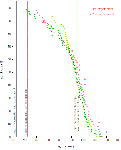This immediately explains why so little life-lengthening gain was seen from so much treatment in the first experiment. Notice that even though the concentration of MePiA used in these two mice experiments—100,000 micrograms per liter of drinking water—is expected to be on the order of 10,000 times larger than the concentration of MePiA naturally available in rainwater thousands of years ago, the life spans of the treated mice in the first experiment were increased only about 20% at best, while the life spans of pre-Flood humans exceeded modern human life spans by at least 1,000%. The reason for this now seems clear. Chronic toxicity of megadose MePiA counteracted the life-lengthening effect of vitamin MePiA.

In hindsight, it is a good thing that treatment was started as late as it was and stopped as soon as it was in the first experiment. The life-lengthening effect of MePiA might otherwise have gone undetected, cancelled entirely by chronic toxicity.

13.4.2  Correction 2: MePA is Efficacious With Mice

The second mistaken idea was that MePA has no effect on mice. This idea had been seeded by earlier, smaller experiments which had failed to detect any effect with mice, and it had been reinforced by the first, megadose experiment with mice.

Figure 13.5 makes explicit that, contrary to the conclusion of the first experiment, MePA does yield life lengthening in mice.

Figure 13.5: Survival curve datasets for ICR female weanling mice showing life lengthening due to intake of MePA and chronic toxicity of megadose MePA. The daily intake of vitamin MePA was dramatically reduced in the second experiment (0.8 milligrams of MePA per liter of drinking water) relative to the first experiment (0.1 grams of MePA per liter of drinking water), yet life lengthening was greatest with the second experiment, implying chronic toxicity of megadose MePA. Three additional batches of the same type of mice raised in the same lab in previous years but never treated with either MePA or MePiA are plotted in various shades of green as usual to provide a visual reference for gauging life lengthening due to the treatments.

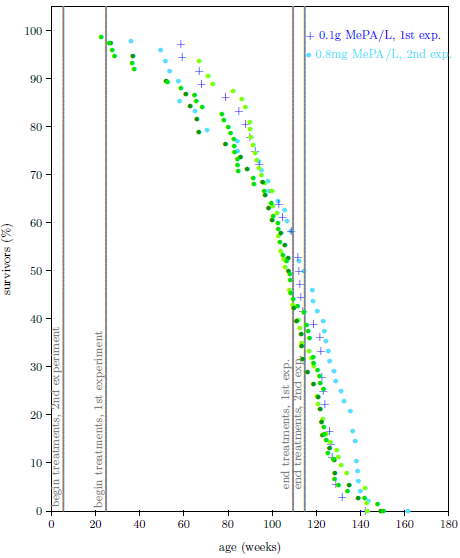This is seen by comparing the MePA mice from the second experiment (blue dots) with the green "control" groups. The second experiment MePA mice (blue dots) life spans begin to exceed the green groups near 60% survivors, and the final survivor of the second experiment MePA mice (blue dots) group displays a maximal life span 11 weeks greater than the maximal life span of the green groups.

MePA clearly results in life lengthening in these mice.

The demonstration, at long last, that MePA is efficacious with mice was not too surprising. MePA use with human volunteers had been going on (next chapter) while these mice experiments were happening, and these had given strong evidence that MePA was a vitamin. A characteristic of the traditional vitamins is that the vitamin molecule involved is essential for most if not all mammals. It would therefore be surprising were vitamin MePA not efficacious with mice.

13.4.3  Correction 3: Megadose MePA is Toxic

Figure 13.5 also makes explicit the negative consequence of prolonged megadose treatment with MePA.

The two MePA datasets are plotted in different shades of blue. The first experiment treated the mice with 0.1 grams MePA per liter of drinking water—megadose MePA. The second experiment treated the mice with 0.8 milligrams of MePA per liter of drinking water. This is a high concentration (800 micrograms of MePA per liter) compared to the expected natural concentration of 10 micrograms of MePA per liter or less, but it is far from the 100,000 micrograms of MePA per liter of the first experiment.

The fact that the much smaller concentration of MePA used in the second experiment gave life lengthening, while the megadose concentration of the first experiment did not, shows immediately that megadose MePA is chronically toxic. This chronic toxicity masked the life-lengthening effect of MePA in the first experiment.

13.4.4  Correction 4: Vitamin X is a Vitamin Duo

The fact that chronic toxicity masked the life-lengthening effect of MePA in the first experiment reopens the question of which vitamin, MePA or MePiA, is truly vitamin X.

It is now clear that both MePA and MePiA yield life lengthening in mice, thus both must be vitamins. It is also clear that these two vitamins, while differing in their physiological roles, are closely related in many ways. Their respective molecules differ only by the presence of an additional oxygen atom in MePA. Their synthesis and distribution in the atmosphere are similar. Their entrance into the human diet pre-Flood via drinking water from ponds, lakes, and rivers is identical. The ease with which MePiA may be converted into MePA portrays an intimate relationship. And, most importantly, both disappeared together from the environment as a result of Noah's Flood since both are products of the same lost precursor gas, MeP.

It thus became clear that, rather than choosing one or the other of these two new vitamins to be vitamin X, it was necessary to discard the notion that a lone vitamin should be found and to embrace the idea that vitamin X was, in fact, a vitamin duo encompassing both MePA and MePiA.

13.5  The Theory of Modern Human Aging

This terminated the working hypothesis that modern human aging results from inadequate dietary vitamin X. Its job was done. The time had come to revert back to the full central hypothesis.

The central hypothesis may now be presented in the following, more focused form: modern human aging is a nutritional deficiency disease resulting from dietary insufficiency of a previously unknown MePA/MePiA vitamin duo made globally deficient by the impact of Noah's Flood on earth's environment.

This immediately rendered obsolete Harman's Theory of Aging, and my Vitamin MePiA Theory of Aging built upon Harman's theory. These theories picture modern human aging as due entirely to a single physiological agent: ROS damage to mitochondria. The General Theory of Aging does not endorse this limited vision. It unifies aging around the single concept of congenital disease, not around a single physiological agent. It specifically allows multiple agents contributing multiple congenital diseases to aging in the general case.

It is now clear that modern human aging involves two physical agents: vitamin MePA and vitamin MePiA. Each contributes its own congenital vitamin deficiency disease, with its own burden of morbidity and mortality.

To capture these fundamental concepts, it is necessary to move on to a more comprehensive theory of aging. I will call this simply the Theory of Modern Human Aging.

Theory of Modern Human Aging: Modern human aging is a congenital nutritional deficiency disease of two newly-discovered, closely-related vitamins: methylphosphinic acid (MePiA) and methylphosphonic acid (MePA). Vitamin MePiA functions as an antioxidant within the mitochondria, protecting them from damage due to ROS. Vitamin MePA functions as its own unique vitamin, separate from vitamin MePiA. It is involved in multiple biochemical pathways, similar to members of the traditional vitamins.

13.6  Conclusion

MePA and MePiA are best thought of as a vitamin duo. Both play a role in MHA. Loss of the MePA/MePiA vitamin duo from the environment as a result of Noah's Flood explains why modern human life spans are less than 125 years while pre-Flood human life spans were greater than 900 years.

Chapter 14

Early Experiences With MePA

For several years, before the final result from the first MePA versus MePiA mice experiment proved otherwise, MePA was thought to be the lone vitamin X. As a result, MePA was tested by itself, first by myself, then by my wife, Helen, and then by other early volunteers. In consequence, the effects ascribed to MePA in the present chapter are, in fact, known to be due to MePA alone and not due to the second-discovered anti-aging vitamin, MePiA.

This could not be done to people today—withhold one deficient vitamin while administering another deficient vitamin. The administering of one deficient vitamin is better than the administering of no deficient vitamin, but knowledgeably withholding any deficient vitamin would be unethical. Humans, uniquely made in God's image (Genesis 1:26–27), are not to be treated like lab animals, and "good science" must give way before human ethics. The results shared in the present chapter are therefore singular and irreplaceable.

14.1  Assessing Benefit Versus Risk

I first identified MePA as a vitamin X candidate, after many false starts, in September of 2014. I began computer modeling work on MePA in June of the following year. By late November 2015, tests with mice to that point had revealed no signs of toxicity, and the theoretical case for MePA had become sufficiently strong to warrant testing it on myself.

It seemed clear that the risks of not beginning to take this compound were at least as high as any risks which might possibly be associated with taking it. I was reasonably sure by that time that MePA had been naturally present in the environment and everybody's diet for time out of mind prior to its gradual loss which began in consequence of the Flood five and a half thousand years previously. This meant that I did not need to worry about it being like a new synthetic compound, totally foreign to the body, with potentially disastrous consequences.

My daily intake—1 microgram per day—would be miniscule. It seemed unlikely that many even synthetic compounds, chosen at random, would be able to do a body much harm at that low intake rate. To get a feeling for the low risk associated with such a small intake, compare, for example, the deadly synthetic compound sarin, "used as a chemical weapon due to its extreme potency as a nerve agent."^[47] A single dose of 500 micrograms—still tiny, but 500 times larger than the intake of MePA I would be taking—administered to a healthy male volunteer caused only "mild symptoms of intoxication."^[48]

Meanwhile, I was approaching 61 years of age. My body was making it increasingly clear that I had passed the plateau phase of the human survivorship curve and that I was rapidly on my way down its precipitous slope.

14.2  MePA Versus "Old Age"

My own mortality had first begun to register with me when I had been forced to get prescription glasses early in my forties. I had always kept myself in reasonably good shape, without getting fanatical about it. I had never smoked, and I had stayed clear of alcohol. My wife and I had walked two miles or more together each day for decades, and I had found little trouble maintaining a healthy weight. But declining eyesight was just the beginning.

Subsequent years brought significant loss of hearing, hypothyroidism, worsening migraine headaches, and more. I had spent a great deal of time studying "old age." Now I was getting to experience first hand what I had studied.

14.2.1  CIDP

The biggest age-related health problem struck just after I turned 50. It began with random pains, short in duration (one or two seconds) but intense, like being stabbed with a needle. I had these in a variety of locations, mostly extremities: thumb, big toe, etc. They seemed not to hit the same spot twice. I shrugged them off. Life was too short and its mysteries too absorbing to be distracted by petty annoyances.

Then, while raking gravel in the driveway, I found I was unable to maintain my grip on the rake handle. Peripheral weakness continued to spread over the following weeks, and then months. It would come and go, but each time it returned, it would be worse than before and stay longer.

After a couple of years of following false leads, I was finally diagnosed with CIDP (chronic inflammatory demyelinating polyneuropathy) by a talented neurologist. CIDP is a rare disease (a few per hundred thousand), most common in men over age 50.

CIDP is an autoimmune disease. The immune system attacks the myelin sheath surrounding nerves. The result is loss of nerve impulses to peripheral muscles, with ensuing weakness.

By the time I got the diagnosis, I was in very bad shape. I was having difficulty lifting my fork to feed myself, I could not button my shirt, I couldn't walk up or down stairs unassisted, and I was worrying at night about smothering under the blankets because I lacked the strength to move them off of my face.

While CIDP cannot be cured by modern medicine, its symptoms can generally be treated and controlled. Over the better part of the next decade, I went through several treatment regimens, from high prednisone to IV-Ig to Hizentra^® home infusions, 60 ml twice per week. Relief of symptoms provided by treatment was not total, but it was nonetheless substantial, allowing me to live a somewhat normal life once again.

Eventually, I was able to resume walking two miles each day with my wife, Helen. But my leg muscles were no longer what they had been. They would rapidly grow weary and pretty much give out after the first mile. No amount of conditioning or exercise helped, so I began taking a bike with me. I would wheel it along beside me as I walked the first mile. It functioned as somewhat of a welcome "walker," keeping me more stable on my feet. Then I would ride it beside Helen as she walked the second mile.

I started taking MePA at 1 microgram/day on November 26, 2015. Three and a half weeks later, I was noticing positive health effects. Most significantly, I began to feel that I could do without the bike on our daily walks. I tried it and, sure enough, I could walk the entire two miles! CIDP had clearly begun to let up. This was eleven years after I had felt those first stabbing pains and subsequent peripheral weakness.

Another two weeks later, I was able to stop the biweekly infusions for CIDP that I had been obliged to be on for years. I had tried coming off the treatments in the past, only to be forced back on them if I wanted to stay out of a wheelchair. Had MePA healed my CIDP?

There were other possibilities. Spontaneous remittance is a characteristic of CIDP in the early years. But I was no longer in the early years. I had not experienced any spontaneous remittance since the relapse that nearly put me in a wheelchair prior to diagnosis. That had been nine years ago. One research study, aimed at assessing the long term prognosis of CIDP, concluded that prognosis "may be determined by the course and response to treatment in the first five years."^[49] Based on the normal progression of this disease, remission seemed most unlikely. And the timing seemed just too coincidental. Remission had begun three and a half weeks following start of MePA intake, after nothing but relentless disease for years.

Another possibility was the well-known placebo effect. But this, too, seemed pretty unlikely to me. Following eleven years of disease, I had expected to have CIDP for the rest of my life. I had always regarded it as possible that vitamin X might reverse CIDP, but I had not regarded this as probable. CIDP is an age-related disease. Age-related diseases are results of MHA. It was clear from the start that, in the process of rolling back MHA, vitamin X might also roll back some age-related diseases. In my case, that meant that it might roll back CIDP. But through the years, when Helen and I had discussed the possible impact on CIDP of the yet-to-be-discovered vitamin X, I had expressed my sincerely held doubts that it could impact diseases of the immune system. I had started on MePA in this frame of mind. My purpose had been to halt "aging." Remission of CIDP had come as a bit of a (pleasant) surprise.

What was needed, to know for sure what was going on, was a proper clinical trial involving both treated and control groups. But all I had was myself. So we waited. Neither placebo effect nor spontaneous remittance would be expected to last more than a few weeks.

It has now been over seven years, and there has been no looking back.

I don't often think about CIDP since its cure. A few years back, while rummaging around on my computer, searching for a file from long ago, I bumped into a checklist I had drafted for Helen and myself for administering home infusions for my CIDP. Suddenly, it all came flooding back. The checklist was a full page long. The needed infusions took Helen and me several hours to carry out, twice each week.

The infusions were a net blessing, of course. They enabled me to have the strength I needed to button my shirt, feed myself, get out of a chair unassisted, navigate the two porch steps without peril of winding up in a broken heap at the bottom, and walk up to a mile unassisted.

But what a great blessing now, to have all this and more—I can even jog or run whenever I feel like it—with no infusions. It is wonderful not to have to plug those four hypodermic needles into my flesh twice each week. It is wonderful to do as I now please with the hours the infusions previously claimed each week. I am tremendously grateful that my CIDP has been cured, restoring me to a level of strength normal to healthy males in their sixties.

14.2.2  Skin

At the same time as CIDP was beginning to let up, I noticed that my skin was becoming more moist and supple. I'd had pretty severe eczema as a child, and my skin had tended to be dry and scaly into adulthood. The evident change for the better with my skin, together with the letting up of CIDP, got me really excited, because I knew that one of the symptoms of hyperthyroidism is oilier skin. I had been obliged to start taking levothyroxine for hypothyroidism early in my fifties. It seemed possible that MePA had begun to heal my thyroid, so that normal supplementation with levothyroxine was now causing hyperthyroidism.

I expected the next regularly scheduled blood test to come back showing high TSA. It came back normal and has remained normal. So MePA has made no discernible difference, so far, to my "worn-out" thyroid gland. Nonetheless, my skin has definitely improved.

I had always regarded a hot bath or shower as one of modern life's few affordable, worthwhile luxuries. I did some of my best thinking in the shower. But after age 50, I had found it increasingly necessary to stay out of the bath and out of the shower. The hot water would make my skin dry, rashy, and miserable the following day.

This too has now reversed. I am able to enjoy the luxury of a hot bath or shower pretty much as I please once again.

For a few weeks during the summer of 2018, my eczema flared up again, following many trouble-free months. This was confusing. Up until then, the vitamin seemed to have made eczema a thing of the past for me. Why had it returned, why in the summer when winters were always previously the worst months, and why had it returned with such stubborn ferocity?

Eventually, I was able to figure out that consumption of an abundance of fresh garden tomatoes was the culprit. When I eliminated tomatoes and citrus (both are reported to contain salicylates and amines, which trigger eczema in some individuals) the problem rapidly cleared up.

In hindsight, it seems clear that MePA allowed my skin to be sufficiently normal, for the first time in my life, for me to be able to figure out that I am allergic to tomatoes and possibly also to citrus.

14.2.3  Sleep

Once I had begun to take MePA, I also found that I was sleeping better. It is easiest to describe the change which took place as simply a return to a more youthful sleep experience. Sleep was deeper and less interrupted. I needed less sleep, and I felt more rested.

Sleep still continues to be of higher quality than it was before the vitamin. I continue to need less sleep, giving me more usable hours in a day. I rise feeling ready to get to work. For the first few years after beginning to take MePA, I would sleep soundly for seven to seven and a half hours, waking once to go to the bathroom. Then the frequency of early morning insomnia began to increase. This seemed to result from sleep having been so sound and refreshing in the first half of the night that the need for sleep was substantially diminished in the second half of the night. Being doubtful that a mere four or five hours of sleep per night could be sufficient, I deliberately kept myself as somnolent as possible when I got up at night, by, for example, using a dim night light in the bathroom, and refusing to let my thoughts focus on anything disturbing or absorbing.

Eventually I found that a routine of office work in the mornings (when my mental faculties are at their best) and physical activity in the afternoons greatly reduced early morning insomnia. A final helpful discovery was that early morning insomnia is markedly reduced by a personal ban on the news media in general. In hindsight, this makes sense. The news industry is profit driven. Profits are highest whenever listeners are kept anxious over what might happen next so they keep coming back to hear more. Anxiety fuels insomnia. I tune the industry out and am rewarded with full nights of deep sleep.

In sharp contrast to pre-vitamin days, when insomnia now occurs, it does not leave me exhausted and unable to get much done the next day. It is as if the half-night's sleep I did get was enough to see me satisfactorily through the day. And I have found that I frequently sleep the whole next night soundly and without difficulty.

The knowledge that I can now get by for a day on very little sleep, and that I will make up for lost sleep the next night, reduces frustration and apprehension if I find myself awake in the early morning hours when I feel I should normally be asleep.

Most recently, I have begun sleeping more hours per night (8 or even 9). As a young person, I had needed 10 hours of sleep per night in order to be functional the next day.

14.2.4  Headache/Migraine

My experience with headaches and migraines stands in stark contrast to what I had been experiencing immediately prior to beginning to supplement MePA.

When I was young, headaches were few, and I could count on a night's sleep to cure a headache completely. As the years passed, I became increasingly susceptible to headaches, and my body became less and less able to cope with them. If I went to sleep with a headache, for example, it would still be with me when I awoke the next morning.

My earliest recollection of a severe headache goes back to my mid thirties. By my mid forties, I was experiencing occasional migraines. All of this was compounded in my mid fifties by treatments for CIDP, of which headaches are a known side effect. Immediately before I started on MePA, when I was nearly 61, I was subject to headaches on a fairly regular basis. These would develop into full-blown, excruciatingly painful migraines if I failed to intervene.

I had learned to take action against headaches as soon as I noticed one beginning. I would take two extra-strength, over-the-counter pain relievers to knock out the headache before it had a chance to get going. The frequency of this corrective/preventive action had increased to an average of roughly once per two weeks. I kept a supply of pain pills in my office, in my vehicle, and near my bed.

This all changed for the better when I began supplementing my diet with vitamin MePA. The frequency of headaches rapidly declined. At present, the most accurate description of my headache frequency is "almost never."

14.2.5  Upper Respiratory Infections

Common upper respiratory infections rapidly reduced in frequency and severity once supplementation with MePA began. The same is true of the stomach flu. I had been living in increasing dread of these common ailments prior to MePA. I was beginning to understand how elderly persons might die of them. I am now back to taking upper respiratory ailments pretty much in stride. I can still catch a full-blown cold or flu and have it take a week or ten days to clear out, but this is relatively rare. More common is to get just a touch of the cold or flu, with symptoms totally resolving in under 24 hours. In the several instances of exposure to stomach flu which I experienced after starting on MePA, only brief, slight nausea resulted.

14.2.6  Helen Corroborates My Early Experience

Coming off of twice-per-week 60 ml infusions of Hizentra^® for CIDP complicated the question of what changes were due to MePA.For this reason, in the early years, before we had testimonials from any other users of MePA, the experience of my wife, Helen, was especially helpful.

Helen began taking 1 microgram MePA/day after I had been taking it for a year with no adverse side effects. She had lived close up with my CIDP for enough years to know that something real had happened. And she was concerned for her own future health, being aware from my research that MePA would not suddenly erase her own rapidly accumulating "old age" symptoms and debilitations.

Three weeks later, she began reporting greatly improved sleep. Previously, she had been experiencing chronic sleep trouble. A typical morning had begun with, "I slept so terribly again last night, I don't know how I can keep up, feeling like this…" Now she was saying, "I haven't slept like this in years." Our grown children began to comment on her remarkably improved ability to cope with life when they came home to visit. She would reply, "Yes, what a difference a good night's sleep makes!"

Helen also corroborated the increased skin oils. In her case, the change was not so welcome as it has been for me. Her skin has always been pretty normal—definitely youthful compared to mine. The practical impact for her was that she had to begin washing her hair three times per week instead of two.

14.2.7  Rate of Healing

Another improvement is that we seem to heal more quickly. For example, I developed very sore muscles in my back between my shoulder blades, and opposite that on my front side, from a bunch of heavy lifting I had to do, on top of some unusual hand pulling of plants I had been obliged to tackle in the garden. The pain was of the sort which takes your breath away. I took nothing for the pain, and I did not treat the sore muscles in any way, which is pretty standard practice for me. I went to bed expecting to lose a lot of sleep due to pain whenever I rolled over. From years of previous experience, I expected at least three days of pain, followed by a week or two of slow healing of residual soreness. What happened is that I slept better than expected, and I woke up with only slight twinges of pain left. By that afternoon, even those were gone.

As another example, I accidentally mashed the end of a finger between two steel pipes. The right half of the fingernail rapidly turned dark purple. It was pretty painful all that day. I wondered whether the purple half of the nail might separate from the finger. But the next day, only a thin purple line remained under the nail, and there was only slight residual pain. The following day, it was difficult to distinguish the finger I had injured from neighboring fingers.

The blessing of rapid healing also shows up repeatedly after a day of strenuous physical work or other unaccustomed physical activity. It was common, prior to the vitamin, to wake up the next morning with aches and pains. These would typically take several days to resolve. Now, when I wake up the next morning, there are no aches and pains.

I do not want to give a wrong impression. It is still possible for some injuries to take time to heal. As an example, about half a year ago, I had a bout of pain in my right hip, causing me to walk with a limp. This was caused by dragging a number of heavy objects across the ground a considerable distance. I seemed to have injured some tissue in my hip joint in the process. The pain would be aggravated by climbing stairs or by peddling a bike. A deep squat would set things right for a while, relieving the pain. This particular injury took a full six weeks to heal.

It had no sooner gotten better than my left hip started acting up. This resulted from repeated trips up and down a long flight of stairs carrying some heavy loads. I thought I was in for another six weeks of pain and limping, but it resolved in a little over a week.

The norm has shifted from slow healing all my life before vitamin MePA to rapid healing since starting to take vitamin MePA, making the six-week hip episode to be noteworthy as a rare exception.

14.2.8  Weight

I made my weight a personal priority a year or so after starting on MePA. Proper weight pays back well for all the discipline it costs—health risks due to excess weight are well known.

I went to the Internet to learn my healthy weight range and my "ideal" weight. This gave me a target of 150 to 155 pounds, at the center of my healthy weight range. I was in the low 170's when I started. I used a calorie counter on my computer to count calories every meal. I adjusted my daily calorie allotment to lose just a half pound per week—I did not want to feel hungry (it is too distracting when I am working), and vitamin MePA seemed to promise a lengthy future, so there was no rush. I soon settled comfortably into my 150- to 155-pound target range and shortly thereafter stopped using the calorie counter. This has resulted in staying around 157 to 158, which I am content with.

I had tried, unsuccessfully, to lose weight prior to starting on vitamin MePA. I credit the vitamin, not with making it easier to lose weight, but with providing the mental energy, resolve, and fortitude needed to make the slow transition to a healthier way of eating.

14.2.9  Arthritis

Helen had suffered from arthritis for years. At present, she is pretty much free of this disease. We tend to forget what an increasingly nagging nuisance it once was.

Arthritis resolves relatively slowly with MePA. In mid 2017, after having been on vitamin MePA at 1 microgram per day for half a year, Helen had noticed no relief from arthritis. But by late 2018, two years and a month after beginning MePA, and having increased her daily intake to 8 micrograms per day, she was reporting significant improvement:^[50]

I used to have constant hip pain [due to arthritis] on my left side, with it being worse at night. The pain is now completely gone, even though I'm on my feet much of the day.

The swollen arthritis in my hands has gone down quite a bit, and I no longer have pain in my hands. Several of my fingers have straightened out now that the swelling has gone down.

The experience of my older sister, Valorie, another early user of MePA, confirmed that healing of arthritis is relatively slow.^[51]

The arthritis in my joints cleared up after ten months of 2 micrograms per day of MePA.

Also, my knees were starting to have problems, which I figured would lead to knee surgery eventually. That has also entirely cleared up.

Helen struggled on and off for several years with neck pain which seemed to be due to arthritis, and also with bursitis for many years. The bursitis took the longest time to resolve after beginning to take MePA. It was still acting up two years later. But at present, neither arthritis nor bursitis has been a problem for a very long time.

14.2.10  More Observations from Helen

Here is more of Helen's experience, shared in late 2018:^[52]

The most noticeable change for me has been my energy level. I have always had high energy, but now I seem to have super high energy. I work typically 12 to 14 hours each day in our home businesses, going at a pretty high speed all day until late evening, when I drop into bed exhausted and sleep soundly.

I notice that I can multitask at a much higher level than before the vitamin. I am busier than I have ever been in my life, which is saying something for a woman who has raised and home schooled ten children. I am wearing many hats, yet I seem to be able to handle the stress of piles of work on my desk just fine. Before the vitamin, I frequently exclaimed (mostly to myself), "I can't DO all of this!" Now, I am able to realize that what doesn't get done today will get done tomorrow. I was never like that; I had to get my desk cleared off every day, or I was stressed—which meant I was often stressed!

The vitamin reduces work-related anxiety. I have much less anxiety now even when in high stress situations. Before the vitamin, when there was a large stress load, I would stay awake for hours at night, sometimes for several nights, "playing the tapes" over and over in my mind. Now I may lose a few hours of sleep, but I am able eventually to relax and go to sleep even though the stress level hasn't reduced. Even when the workload is extremely heavy, I am able to handle it just fine.

It is hard to describe the feeling I have of psychological wellness—the feeling of being able to handle whatever life throws at you. As you can imagine, with ten children and 26 grands plus several growing businesses, I feel like I get thrown the occasional hard and fast curve ball. I am now able to somehow put things in proper perspective and move on much quicker than I had been able to before the vitamin.

I am able to handle company much more now, and even welcome it! I enjoyed having company when I was younger, but in the years just prior to the vitamin, I was dreading having company more and more, even family, and I tried to get out of having company as much as I could.

Thanksgiving 2018 had me decorating, cooking, cleaning, organizing a large children's treasure hunt, door prizes, and the like with great enthusiasm despite the heavy workload due to growth in our various home businesses. I'm very excited about Christmas 2018 and am already decorating. (In the past I would normally not decorate until a few days before Christmas, and it would usually be minimal.) This year, I am having a family open house in our home for several events over the holidays.

I can get away with less sleep, feeling ready to get up after about 5–6 hours of heavy sleep. I find that I'm dreaming a lot more, especially in the early hours of the morning. Even if I have a bad night's sleep, for whatever reason, I'm still able to work hard and generally have no need for an afternoon nap.

The age spots on the left side of my face are almost gone, and the other aging spots on my face are fading slowly.

I am still having to wash my hair about every 2 to 3 days as it is much oiler than before the vitamin.

My eyesight seems the same; I still need glasses, sadly.

My eyebrows and hair have thickened. I was always losing hair before taking the vitamin. It is now thicker, like it was when I was a much younger woman. My gray hair is still there. My hair doesn't seem to be getting grayer, but the amount of gray is a hard thing to measure.

I notice that if I get injured in some way, like a cut on my hand, or a bruise from falling, then healing is rapid and almost unreal. The next day, after the injury, it seems totally healed.

The truth is, I have always felt younger than my age. But now, at 64, I feel like I'm in my 20's.

For example, I have always wanted to have a straight (pencil) jean skirt. I had been watching for one in the thrift store for a year or so and finally found one. I was so excited and could hardly wait to wear it. I put it on one morning, and got to work in the shipping room packing boxes for mail orders. But it was just not practical—one cannot run in a straight skirt!

Even though I am a grandmother many times over, I don't spend much time on the porch in a rocking chair!

From time to time, Gerald comments, "You're a new woman." He's right!

14.3  Conclusion

We now know that MePA is just one part of the anti-aging vitamin story. Vitamin MePiA must also be taken into consideration. But the impact of MePA alone on my personal health and on Helen's personal health has been enormous. I believe that it is probably the case that I would be dead by now were it not for the discovery of MePA. I was rapidly declining in overall health and robustness prior to beginning supplementation of my diet with vitamin MePA. So many negative "old age" health effects which had set in and become what seemed to be a permanent part of my remaining life back then have now been swept away. Helen's experience has been the same. Our resilience is much increased, and our quality of life is so much better than it was for both of us before we first began dietary supplementation with vitamin MePA.

Chapter 15

Vitamin MePA

15.1  MePA–a New Vitamin?

The early 1900s were the golden years of vitamin discovery. The last of the thirteen traditional vitamins was discovered in 1948.

I was born in 1955. Vitamins were still a subject of topical interest—even faddish—in ordinary circles when I was a child. Every young housewife knew the importance of seeing to it that her family got their needed vitamins. One of my most unpleasant childhood memories is having to take cod liver oil, spoon fed to me and my siblings by Mom to help us get our vitamins.

By the time I had discovered MePA, vitamins were no longer fashionable in everyday conversation, and childhood memories had faded significantly. It seemed by that time that the age of vitamin discovery had long ago ended, making improbable the postulate of discovery of a previously unknown vitamin.

Starting out, nothing was known about the physiological properties of MePA. It was deemed to be a vitamin because that is what the central hypothesis called for. But, once research related to dietary use of MePA had begun, evidence rapidly accumulated verifying its vitamin status.

15.1.1  Anti-aging Vitamins Predicted

Casimir Funk, whom many regard as the "father of vitamin therapy,"^[53] observed in 1949 that:

The study of degenerative pathological changes of old age… may well belong to a future chapter of vitamin research.^[54]

Figure 15.1: Niacin (vitamin B₃) deficiency disease (commonly known as pellagra) in a 6-month-old pig (left) and the same pig 3 months later after having been fed the same diet but fortified with niacin (right). The geriatric features of the 6-month-old pig were a result of its niacin deficiency.^[55]

By definition, a molecule is a "vitamin" depending on what it does, not on whether it is listed as one of the thirteen traditional vitamins. This is necessary because the thirteen traditional vitamins were discovered over a protracted period of time, and there has never been any scientific reason to suppose that the discovery process has ended or that the traditional thirteen vitamins exhaust the vitamin category.

15.1.2  MePA Behaves Similar to Other Vitamins

Dietary supplementation with microgram per day amounts of MePA has been found to relieve symptoms of many age-related ailments, implying that MePA operates in its own biochemical pathways within the body in a typical vitamin capacity.

MePA, a water-soluble weak acid, behaves in a way which is characteristic of the water-soluble vitamins in general. Compare it to dietary supplementation with niacin (or nicotinic acid), another water-soluble weak acid, for example.

Clinically advanced pellagra is rare in the U.S. today, but before the discovery of nicotinic acid in the latter half of the 1930's, pellagra was common in the southern states where corn was a major staple in human diets. Following is a description from back at that time^[56] of the effects on pellagra patients of treatment with nicotinic acid.

A comprehensive report has been made by Spies, Bean, and Ashe, based on observations at the Cincinnati General Hospital, and the Hillman Hospital, Birmingham, Alabama, on the nicotinic acid treatment of hundreds of cases of classic pellagra. It is stated that:

"The administration of adequate amounts of nicotinic acid or one of its compounds is followed by the disappearance of many symptoms of the disease. Within 24 to 72 hours [1 to 3 days], the fiery redness and swelling of the tongue, gums, mouth, throat, and vagina subside, and the associated Vincent's infection disappears. Within 24 to 72 hours, nausea and vomiting cease, the increased salivation decreases, and bowel movements become normal. Abdominal distention, pain and discomfort disappear and, in most cases, the desire for food returns. The acute, fiery red erythematous [reddening of the skin, usually in patches] dermal lesions, in which the epithelium [thin tissue forming the outer layer of a body's surface] is intact, blanch within 48 hours after the administration of nicotinic acid, but where the continuity of the skin is broken and the lesions are moist, ulcerated, dry or pigmented, there seems to be no specific benefit. Perhaps the most dramatic response of the pellagrin to nicotinic acid therapy is the disappearance of the acute mental symptoms. These symptoms, varying from slight confusion to delirium and mania, disappear rapidly, often over night. The maniacal patients become calm and the confused patients, mentally clear. After therapy they become readjusted, and often have excellent insight and memory of their actions, ideas and surroundings during the psychotic period. Apathy and lassitude give way to interest."

Relief of diverse symptoms with no hint of any negative side effects due to treatment is characteristic of the cure of a deficiency disease by a water-soluble vitamin. This same behavior is seen with MePA. Following is a summary of experience gained to date with volunteers taking MePA in microgram amounts per day, deliberately imitating the form of the report on the nicotinic acid treatment of pellagra cases quoted above, to show the similarity of the two cases.

A compilation of testimonials has been made by Aardsma at https://agingcauseandcure.com/summary-reports/ on the methylphosphonic acid treatment of dozens of cases of MHA. It has been found that:

The administration of adequate amounts of methylphosphonic acid (MePA) is followed by the disappearance of many symptoms of the disease. Within a few weeks to a few months, the sleep disorders characteristic of aging subside: there is less trouble getting to sleep (i.e., reduced insomnia), sleep is deeper and more refreshing, and less sleep is needed. Associated fatigue is reduced or disappears. The rate of wound healing is remarkably increased, and accompanying inflammation and pain are decreased. The incidence of headaches and migraines is reduced. Within a few weeks to a few months, diseases which have taken hold because of agedness, such as heart failure, cancers, and autoimmune disease, may begin to be slowed, reversed, or cured. Numerous skin disorders disappear: skin becomes more moist and supple; chronic skin infections begin to clear up within a month after the administration of methylphosphonic acid. Perhaps the most dramatic response of the elderly to methylphosphonic acid therapy is the disappearance of chronic mental symptoms. These symptoms, varying from "brain fog" to depression and anxiety, disappear rapidly, sometimes within the first week. The depressed become more happy, the anxious, more calm, and the "brain fogged," mentally clear. Apathy and lassitude give way to interest and creativity.

15.1.3  MePA is Vitamin-Like, Not Drug-Like

Additional evidence indicating that MePA is a vitamin is provided by the observation that the physiologically active intake range is very low, and, simultaneously, its toxicity is also very low. This is a distinctive characteristic of many of the vitamins, with 6 out of the 13 traditional vitamins having microgram per day recommended intakes but limited toxicity.^[57]

Vitamin B₁₂ is a particularly striking example. Vitamin B₁₂ has the lowest recommended daily intake of any of the vitamins (2.4 micrograms per day for an adult male) but has no apparent oral toxicity in humans.^[58] In mice, its acute oral toxicity exceeds 5 g/kg body weight (BW).^[59] To put this in perspective, assuming the same toxicity level, the safety margin is 152 million for a person weighing 73 kg and taking 2.4 micrograms of vitamin B₁₂ per day.

The physiologically responsive range for MePA is on par with that of vitamin B₁₂, with intakes as low as 1 microgram per day eliciting marked physiological response. When an LD50 (lethal dose, 50%) of 1888 mg/kg BW^[60] is used in conjunction with a recommended daily intake of 10 micrograms per day, the safety margin for intake of MePA is 14 million.

These very low recommended intake levels coupled with very large safety margins for vitamin B₁₂ and MePA are not characteristic of most drugs. Most drugs require intakes in the mg per day range in order to elicit the desired physiological response. There are, however, a limited number of drugs that are capable of a physiological response at very low doses. For example, the drug carfentanil can elicit a response in humans starting around 1 microgram.^[61] However, a general characteristic of these extremely potent drugs is that the range of safe intake levels around the physiologically responsive range is very small. For example, while human toxicity data is limited, carfentanil is potentially lethal at a dose of 20 micrograms.^[62] Thus, the safety margin for intake of carfentanil is only about 20 relative to the minimum amount needed to see a physiological response.

While MePA shares its microgram-range-physiologically-responsive-intake property with both vitamin B₁₂ and the drug carfentanil, it does not have the small-safety-margin property of carfentanil, but rather has the large-safety-margin property of vitamin B₁₂. In this respect, MePA is similar to the vitamin, B₁₂, not the drug, carfentanil, thus providing further evidence that MePA is a vitamin.

15.1.4  MePA Satisfies the Criteria for a Vitamin

Four criteria serve to define a vitamin. Vitamins are (1) organic compounds, (2) which must be obtained through the diet, (3) which are vital to the health of the organism, and (4) which are needed in tiny amounts only.

These four criteria, when taken together, are highly restrictive. Of the myriad of molecules known to chemistry, to the present time all have been eliminated from the vitamin category by these four criteria save just over a dozen diverse chemical compounds. That MePA easily fulfills these restrictive criteria is seen as follows:

1. organic compounds
   Organic compounds include carbon in their molecular structure. The methyl group, CH₃, in methylphosphonic acid makes MePA to be an organic compound.

2. which must be obtained through the diet
   There is no endogenous synthesis of MePA in the body, with the only organisms believed to have genetic capability for endogenous synthesis being select marine microorganisms.^[63] Since MePiA and MePA are related through oxidation-reduction reactions, generation of MePA within the body from in vivo oxidation of MePiA is theoretically possible. Whether sufficient MePA to meet the body's needs might be obtained in this way from intake of MePiA alone is so far not known. Historically, the natural dietary source for both MePA and MePiA was surface sources of drinking water. Because MePA is the stable end product of MePiA oxidation, MePA is expected to have accumulated in such sources, causing it to have been present at higher concentrations than MePiA in natural sources. In addition, the very long biological half-life of MePiA implies that little of it will be lost to MePA in vivo. Thus, the present state of knowledge renders dubious the idea that sufficient MePA might be obtained merely by intake of natural concentrations of MePiA. It presently appears that adequate physiological levels of MePA require that MePA itself be included in the diet.

3. which are vital to the health of the organism
   Absence of dietary MePA contributes to the morbidity and mortality of MHA. In a subsequent chapter, it will be shown that MePA deficiency disease causes roughly 53% of modern deaths due to all causes in the United States.

4. which are needed in tiny amounts only
   As little as 1 microgram of MePA per day has been found to be physiologically efficacious with an adult male. This is less than one part per billion on a weight of MePA to weight of total food ingested per day basis.

15.2  The Cure for MePA Deficiency Disease

To cure a vitamin deficiency disease requires only adequate intake of the deficient vitamin. Normally, adequate intake of a vitamin is obtained by eating foods containing that vitamin in adequate amounts. This normal strategy will not work with vitamin MePA because there is no natural food or drink which contains this vitamin today.

In the ancient past, this vitamin was naturally available in rainwater. As a result, it was present in the water ancient individuals drank from rainwater-fed sources such as ponds and rivers. But Noah's Flood broke the natural production of vitamin MePA so that it is not available in rainwater-fed sources of drinking water any longer.

To obtain an adequate daily intake of MePA today, it is necessary to supplement one's diet with this vitamin artificially. The chemical compound corresponding to vitamin MePA is methylphosphonic acid. This is a known chemical compound, used in industry, making it readily available commercially. As a result, supplementation of diets with vitamin MePA may be easily accomplished today.

People supplementing their diets with MePA report many and varied health improvements.^[64] For this reason, vitamin MePA, while certainly not a panacea, may be regarded as the "general health" anti-aging vitamin. Vitamin MePA appears to be involved in multiple biochemical processes in the body—as is true of most of the vitamins—so that, in its absence, multiple things go wrong in the body and multiple ailments result. The negative health consequences of MePA deficiency disease are not trivial. They contribute a large load of morbidity and mortality to "old age" in modern humans.

Experience with MePA deficiency disease to date indicates that healing of MePA deficiency disease is relatively prompt—days, weeks, or months for most symptoms once adequate daily intake has begun.

15.2.1  Recommended Daily Intake

Recommended Daily Intake or Reference Daily Intake (RDI) is the normal metric used by nutritionists seeking to establish an appropriate consumption level of a given vitamin or other nutrient. Determination of the optimal daily intake of any vitamin is not a trivial exercise. Although the chemical compound corresponding to vitamin C, ascorbic acid, was discovered in the 1930's, the optimal daily intake is still an ongoing debate today.

The appropriate daily intake is still vigorously disputed by scientists, and recommended allowances not only vary from one country to another; they also change from time to time within the same country. Although everyone agrees that the minimal daily requirement for vitamin C is 10 mg or slightly less, there is little agreement regarding recommended intakes.^[65]

To guarantee dietary sufficiency, 20 micrograms MePA per day for adult males was recommended for several years.^[66] Direct measurement of MePA excreted in the urine of a human volunteer supplementing her diet at that recommended daily intake (RDI) level was accomplished in June, 2022, enabling this recommendation to be halved.^[67] While continued refinement of the RDI for MePA seems likely in the future, there is no concern either for efficacy or for safety at the present RDI, reducing the urgency for further research in this direction.

15.3  Conclusion

The cause of MePA deficiency disease is dietary insufficiency of MePA (methylphosphonic acid), a previously unknown vitamin. Today, because of the absence of MePA in potable water sources globally, dietary insufficiency of MePA is a congenital condition of the global human population. This makes MePA deficiency disease to be an "aging" disease—a universal disease which actively progresses from birth on.

On the basis of the personal experiences with vitamin MePA of myself, Helen, and other early volunteers,^[68] I initiated the patent application process for MePA beginning in July 2017. Subsequently, a regular patent application was filed under the title "Compositions and Methods for Treating Aging and/or Improving Human Health." This was split by the U.S. Patent and Trademark Office examiner into two inventions, one for the composition and the other for the method of this newly invented treatment for aging. The composition patent was awarded as patent number US 10,863,764 B2 on December 15, 2020. The method patent was awarded as patent number US 11,596,166 B2 on March 7, 2023.

The cure for MePA deficiency disease is in hand and is commercially available. The cure is simply daily intake of MePA in adequate amounts. Dr. Aardsma's Anti-Aging Vitamins dietary supplement^[69] makes it easy to obtain an adequate daily intake of MePA.

Chapter 16

Inadvertent Experience With MePiA

16.1  The Difficulty of Crediting Symptoms to MePiA

Because MePiA is a phosphinate, and because phosphinates have limited biological utility, as discussed in Chapter 12, the physiological role of MePiA is expected to be antioxidation alone, and this role seems to be specialized to the mitochondria alone. This focuses attention on the mitochondria in discussions of the physiological impact of MePiA. However, because mitochondria are present in most cells of the human body and because healthy mitochondria are essential to healthy cells, MePiA deficiency disease can manifest itself in diverse symptoms of diverse organs and tissues. Unfortunately, however, it is difficult to credit MePiA deficiency disease uniquely with specific observed symptoms because, in the presence of oxygen, both in vivo and in vitro, MePiA is always accompanied by its oxidation product, MePA. MePA is known to be physiologically active in diverse ways, making it practically impossible to credit a specific symptom to MePiA alone.

For this reason, recent results from an inadvertent experiment with mice have been especially of interest. This inadvertent experiment seems to have isolated the physiological impact of MePiA in one cage of four mice.

16.2  An Inadvertent Experiment

The cage of mice in question belonged initially to the MePA mice of the second experiment reported on in Chapter 13. Recall that these mice were administered sufficient MePA from weanling at 5.4 weeks to "old age" with roughly 50% survivors at 114.7 weeks (Figure 13.3). This cage of mice was excluded from the results for this group discussed and plotted in Chapter 13.

The background to this cage of mice—cage 23—is somewhat embarrassing.

It fell to my lot to have to look after the ARP Rodent Lab the week of March 13, 2022. At the time, this lab was under the supervision and day-to-day care of my son, Matthew (PhD, Animal Sciences, Purdue University). Matthew would be taking the week off. Up to that point, the second mice experiment had been expertly taken care of by him. This would be my first time trying to fill Matthew's shoes in his area of expertise in this lab.

Midway through the week, the Rodent Lab routine called for each cage to be changed out for a clean cage with clean bedding, fresh water (containing appropriate MePA and/or MePiA treatment), and adequate food for the week. The protocol was more complex than it sounds, lasting several hours, with several procedures needing to be executed in proper order at the proper place, cage after cage. The weights of the animals and of the food they had consumed had to be measured and recorded, and elaborate attention had to be paid to sanitation and disinfection.

I did pretty well. I made a few minor mistakes, only one of which ever amounted to anything significant. I accidentally supplied one MePA cage with a bottle of MePiA (megadose) treatment. A few minutes later, it occurred to me that I had made this mistake, and I quickly switched the errant bottle for the correct one. Unfortunately, I compounded the mistake (this is the embarrassing part) by failing to note in the lab book which cage this mistake had been made on.

Not long thereafter, Matthew found it necessary to leave ARP for personal health reasons, and the further care and keeping of these mice fell back to me from then on.

As the months passed, and surviving mice in this second experiment became fewer and fewer, I began to notice a strange pattern with Cage 23. While the remaining cages had only one or two mice surviving of the original four per cage, Cage 23 had three mice surviving, and these three mice looked unusually youthful and healthy compared to most of the other surviving mice. I was puzzled and perplexed by this. What was up with these three mice?

As time passed, the anomaly only increased: the surviving mice dwindled to just a few cages of lone, generally very sick-looking and sick-acting "old" mice, but the three mice carried on, looking healthy.

Eventually it came to mind that these second MePA/MePiA experiment mice were the group of mice that I had made the bottle-mixup mistake on. Had the mistake possibly been made on Cage 23? It was at this point that I found that I had failed to record the cage number in the lab book. So all I knew for sure is that I had made the mistake on an MePA cage. Sure enough, Cage 23, with the three anomalous mice, was an MePA cage.

By the time the experiment was nearly over, the anomaly had become stark. In my lab, the record age for this type of mouse not treated with either MePA or MePiA (i.e., for control mice) is 150.4 weeks.^[70] I call mice which live beyond this record age for control mice "long-lived." Four of the 54 MePA mice in this second experiment were long-lived. Three of them were from Cage 23. The life spans of these three mice were 152.3, 158.3, and 165.1 weeks respectively.

I worked out the statistics of having three of four long-lived mice together in one of thirteen cages. I found that the probability of this happening by chance was less than one in one hundred.

It thus appears that, though the wrong, megadose MePiA bottle was in the cage only a short while—probably less than five minutes—at least some of the mice had nonetheless ingested some of the MePiA treatment. The treatment was at megadose concentration, so even a little sip would have delivered a large intake of MePiA. And MePiA has a long biological half-life, as previously discussed. So any mice taking a sip would have benefited from (a slowly dwindling level of) MePiA in their mitochondria long after the sip.

In short, it appears that Cage 23 mice were subject to a unique, unintended experiment. They were treated in every way the same as the other MePA mice in the other 12 cages of their group, except for a five minute exposure to megadose MePiA at 108.7 weeks of age. So they received sufficient dietary MePA and insufficient (in fact, zero) dietary MePiA throughout the treatment interval (i.e., for most of their lives), just like the rest of the group, but the diets of at least some of the Cage 23 mice were very briefly augmented with more-than-sufficient dietary MePiA at 108.7 weeks of age.

16.3  Conclusion

This inadvertent experiment produced three important results.

First, it showed once again that the body is unable to satisfy physiological MePiA requirements from dietary intake of MePA. It seems likely to be biologically necessary that cells not be able to convert MePA to MePiA in a general way. MePA is itself a vitamin necessary for normal metabolism, as discussed in Chapter 15. If cells converted all MePA to MePiA, a cellular MePA deficiency would result. Meanwhile, we have previously seen that the very long half-life of MePiA in the body implies that MePA resulting from free-radical oxidation of MePiA in the mitochondria is likely recycled to MePiA. These considerations imply (1) that conversion of MePA to MePiA happens only in the mitochondria, not throughout the cell in general, and (2) that MePA must not be able to penetrate from the cytoplasm into the mitochondria.

Second, it showed that MePiA boosts health and longevity, as expected, and that it does so even when administered late in life. The accidental intake of MePiA happened when the Cage 23 mice had already reached the advanced human-equivalent age of 86 years.

Third, it emphasized the fact that the "old" look is simply the look of sickness associated with advanced disease. These Cage 23 mice did not look "old" when the rest of the mice in their group looked "old." They still looked young. They only began to look "old" shortly before they died.

These Cage 23 mice thus serve as the best example we currently possess of what may be expected to happen to modern individuals who begin adequate intake of MePiA (e.g, to present users of Dr. Aardsma's Anti-Aging Vitamins). Thanks to this inadvertent experiment, it is now clear that such individuals may be expected to stay healthy longer and live longer than they would have had they not begun adequate intake of MePiA. And some of them may even be expected to break the present world record age of 122 years—the last of these three mice to die had a human-equivalent age at death of 130 years.

These expectations are especially likely to be realized if these MePiA users stick with daily supplementation their whole lives, guaranteeing adequacy of mitochondrial concentrations of MePiA, which the brief intake of the Cage 23 mice would not have guaranteed. And these expectations are yet more especially likely to be realized the younger these MePiA users are when they begin daily supplementation with MePiA.

Chapter 17

Vitamin MePiA

17.1  MePiA is Another New Vitamin

Like MePA, MePiA fulfills the definition of a vitamin: (1) an organic compound, (2) which must be obtained through the diet, (3) which is vital to the health of the organism, and (4) which is needed in tiny amounts only.

1. an organic compound
   Organic compounds include carbon in their molecular structure. The methyl group, CH₃, in methylphosphinic acid makes MePiA to be an organic compound.
2. which must be obtained through the diet
   MePiA must be obtained through the diet. Human bodies cannot synthesize MePiA.
3. which is vital to the health of the organism
   That MePiA is vital to human health is made plain by the biblical historical data showing that life spans diminished—people died at ever lower calendar ages—as its dietary intake diminished. In a subsequent chapter, I will show that MePiA deficiency disease is responsible for roughly 40% of modern deaths due to all causes in the United States.
4. which is needed in tiny amounts only
   Direct measurement of MePiA excreted in the urine of a human volunteer supplementing her diet with 15 micrograms MePiA per day was accomplished in June, 2022, showing that most of the intake amount was being excreted.^[71] It thus appears that the daily need of MePiA is less than 10 micrograms per day.

17.2  The Cure for MePiA Deficiency Disease

Supplementation of the diet with an adequate daily intake of MePiA constitutes the cure for MePiA deficiency disease. The Flood broke the natural supply of MePiA, just as it broke the natural supply of MePA. As a result, to obtain an adequate daily intake of MePiA today, it is necessary to supplement one's diet with this vitamin artificially.

The chemical compound corresponding to vitamin MePiA is methylphosphinic acid. This is a known compound which can be chemically synthesized. As a result, supplementation of diets with vitamin MePiA may be easily accomplished today.

While, as previously mentioned, recovery from MePA deficiency disease appears to be fairly rapid once adequate daily intake has begun, recovery from MePiA deficiency disease appears to be significantly slower. Speaking from my own personal experience as the longest user of MePiA (7 years), augmented by the experience of other early users of MePiA, typical "old age" symptoms not relieved by adequate daily intake of MePA, such as graying of hair and need of eye glasses, seem either to halt (but not turn around) or slowly to progress for some years following commencement of adequate daily intake of MePiA. This observation implies that repair of ROS damage to mitochondria is not a rapid process. The nature of ROS damage to mitochondria is discussed in more detail in the next chapter, providing further insight into this observation.

17.2.1  Recommended Daily Intake of MePiA

In the case of MePiA, one may wonder whether daily intake is really necessary given the very long biological half-life of this vitamin. The short answer is that while daily intake seems unlikely to be necessary, it is nonetheless expedient. Since the biological half-life of MePiA appears to be over a century, it is theoretically possible that weekly, monthly, and even yearly supplementation with this vitamin, at increasingly large intakes as the interval is lengthened, might suffice to meet physiological needs. The main theoretical argument against such a practice is that the natural frequency of intake prior to the Flood was daily—indeed, every time one took a drink of water. The incredibly complex human body is likely to be best served by emulating this natural frequency. In addition, there is a practical argument, it being most convenient to take this vitamin daily together with MePA.

While the need for MePiA is now known to be less than 10 micrograms per day, as mentioned above, determination of the optimal intake of MePiA seems likely to be an area of active research for years to come. The daily requirement may be very small, making direct measurement in urine difficult. It presently appears that life span experiments with mice at different concentrations of MePiA in their drinking water may be the best approach to determination of optimal intake.

17.2.2  Overdosing

Meanwhile, there seems to be less reason for concern about overdosing than there is for underdosing with MePiA. This compound displays low acute oral toxicity.^[72] The results of a study with rats showed an LD50 (lethal dose, 50%) of 940 mg/kg body weight (BW) with a 95% confidence interval of 476 to 1,858 mg/kg BW. This places the acute oral toxicity of MePiA 1.9 times lower than the 501 mg/kg BW minimum required for a compound to be considered to be in the low acute oral toxicity category.^[73]

For general reference on the toxicity scale, comparing oral LD50 values in rats, MePiA is 3.2 times more toxic than table salt (NaCl)^[74], and 4.9 times less toxic than caffeine.^[75]

In addition to being of low acute oral toxicity, MePiA is not mutagenic.^[76]

Water-soluble vitamins, especially those which are small acids, do not generally pose a risk of overdose, as any excess is readily removed from the body by the kidneys. This property seems to be shared, as expected, by MePiA. Tolerance to overdosing with MePiA in humans seems to have been demonstrated by the full life spans enjoyed by both Noah and Shem who lived through the Spike, as well as by the first three post-Flood generations who were born during the Spike. All of these individuals appear to have been subject to very high MePiA intakes during the Spike, and these high intakes seem to have done them no harm, at least as far as longevity is concerned.

Meanwhile, underdosing is known to contribute to the ravages of "old age," dramatically reducing potential life expectancy.

17.2.3  Present Recommendation

With insufficient intake as the primary concern, an initial recommendation of 20 micrograms MePiA per day for adult males was made.^[77] This has now been reduced to 10 micrograms MePiA per day for adult males based on measurement of MePiA excreted in urine.^[78] This recommendation will no doubt be refined further in the future.

17.3  Conclusion

The cause of MePiA deficiency disease is dietary insufficiency of MePiA (methylphosphinic acid), a previously unknown vitamin. Today, because of the absence of MePiA in potable water sources globally, dietary insufficiency of MePiA is a congenital condition of the global human population. This makes MePiA deficiency disease to be an "aging" disease—a universal disease which actively progresses from birth on.

On the basis of the first MePA versus MePiA mouse experiment, I filed a regular patent application for MePiA under the title "Methylphosphinic Acid Compositions and Methods for Reducing Aging" on July 23, 2019. This was awarded as patent number US 11,458,150 B2 on October 4, 2022.

The cure for vitamin MePiA deficiency disease, like MePA deficiency disease, is in hand and commercially available. As with MePA, the cure is simply daily intake of MePiA in adequate amounts.

Dr. Aardsma's Anti-Aging Vitamins dietary supplement^[79] makes it easy to obtain an adequate daily intake of both MePA and MePiA. Since these two diseases comprise MHA, this means that the cure for MHA is also in hand and commercially available.

Chapter 18

Explaining Modern Human Life Spans

18.1  Defining the Problem

Up to this point, ancient biblical life span data have been used first to instigate and then to refine a new theory of human aging called the Theory of Modern Human Aging. The most fundamental postulate of this new theory is that human aging is a nutritional deficiency disease. Initially, it was assumed that aging was the lone disease of a single vitamin, the way scurvy is the lone disease of vitamin C deficiency. Subsequently, it became clear that there are two, previously unknown, closely-related anti-aging vitamins involved: 1) vitamin MePA, and 2) vitamin MePiA. Thus, MHA is a nutritional deficiency disease of two separate vitamin deficiencies combined.

While initial development of this new theory of human aging has relied heavily on ancient human life span data, we are now in a position to see whether this theory is able to explain modern human life span data. The question is not whether the Theory of Modern Human Aging can explain the dramatic shortness of modern human life spans relative to ancient biblical life spans. It does that at the outset. Remove a vitamin from a person's diet and you can be sure that person will die too soon. We modern humans are dying much too soon relative to humans who lived 6,000 years ago because vitamins MePA and MePiA are missing from modern diets. The question is whether this new theory can account for the detailed pattern of modern shortened life spans; the dramatic shortness of modern human life spans is already amply explained.

Modern human life span data reveal a distinctive pattern.

For each calendar year, or cohort, death rates are relatively high in the first year after birth, decline very rapidly to a low point around age 10, and thereafter rise, in a roughly exponential fashion, before decelerating (or slowing their rate of increase) at the end of the life span.^[80]

The purpose, this chapter, is both to test the Theory of Modern Human Aging and to advance understanding of the nature of MHA by using the Theory of Modern Human Aging to model modern, human life span data.

Because much of this chapter is necessarily mathematical, lay readers may wish to skip down to its final Discussion and Conclusion sections.

18.2  The Modern Actuarial Dataset

The data of interest to the present investigation are shown graphically in Figure 18.1.

Figure 18.1: Survival curve data for U.S. males (blue dots) and females (red dots) for the year 2016. Weighted least-squares fit survival curves of the Aardsma model for these two groups are shown in magenta and green respectively.

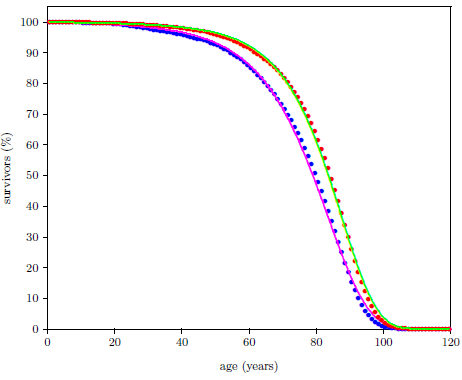This dataset is for the year 2016 from the United States Social Security Administration's list of actuarial life tables.^[81] It is an extraordinary dataset, incorporating death data from 2,744,248 individuals.^[82] This large number of individuals results in very small measurement uncertainties in most of the individual data points, allowing small effects to be clearly resolved.

18.3  Review

The Aardsma model for generic aging disease provides the needed foundation for explaining this dataset. Recall that this model was specified in Chapter 4 as:

In the present context, this equation includes two contributions to death of individuals within a total population of N₀ individuals all of the same age. The first contribution is due to aging disease, controlled by K and A, and the second contribution is due to random extraneous (i.e., not due to aging) events, like lightning strikes, controlled by R.

Figure 18.1 shows that the Aardsma model is able to explain the gross features of the pattern of the dataset reasonably well. That is, the fitted curves follow the data points reasonably well. This says that the modern human survival curve is dominated, in panoramic view, by an incidence of death due to aging which increases exponentially with age.

This same result has already been shown, in Figure 4.2, for the male group data. There, I noted that, while the coarse pattern of the dataset is explained by the Aardsma model, the fine details of the dataset are not explained at all. This is most forcefully revealed by the goodness-of-fit parameter, Χ_ν², for the two curves of Figure 18.1. For a good fit, this parameter is expected to be less than 1.5. For the fit to the male data it is 17,462, and for the female data it is 8,494.

The fits are as poor as they are because, as has previously been pointed out, actuarial life table data include deaths from many other causes than just aging. The Aardsma model includes an age-independent, random deaths term, but it neglects all age-dependent extraneous causes of death. This is suitable for much laboratory animal data, but it is not suitable for real-life human life span data. While laboratory animals do not kill one another in wars, for example, real-life humans do.

18.4  Method

There are two ways to explain these modern life span data quantitatively using the Aardsma model: either 1) upgrade the Aardsma model by adding more terms needed to describe additional causes of death, or 2) eliminate the neglected extraneous deaths from the dataset in some way.

In the following analysis, I will be using the second method. Because the analysis is no longer seeking to explain just the broad outline of the dataset—because it is now digging into the details—this is an unavoidably complex undertaking. To keep things as simple as possible, I will proceed in small steps, chipping away at the analysis a piece at a time, to arrive at a final solution through a series of successive approximations.

18.4.1  Step 1: Model a Single Aging Disease

The Aardsma model, as it is presented in Equation 18.1, describes aging in a generic way. The Theory of Modern Human Aging is not generic. It describes two specific aging diseases—MePiA deficiency disease and MePA deficiency disease—each of which contributes to MHA in its own specific way. Both of these diseases need ultimately to be represented in the model, each by its own individual term patterned on the Aardsma model. As a first step in this direction, include in the model at this stage only a single disease.

18.4.2  Step 2: Fit the First-Approximation Model to the Modern Male Life Span Dataset

The next objective is to fit this first-approximation model to the 2016 actuarial dataset to see how well it does at this level of approximation. To keep things as simple as possible, focus on just the male dataset for now.

It is clear from Figure 18.1 that this simple model does not do well when fit to the entire male dataset, as mentioned above. The presence of age-dependent extraneous deaths within the data is not included in the model. To make progress toward the present objective, a method of eliminating these extraneous deaths from the dataset must be devised.

The Aardsma model already accounts for age-independent extraneous deaths. This is what the R is all about in Equation 18.1. These are deaths that can happen to anybody at any age with equal probability. Being struck by a meteorite is a good, if rare, example of an age-independent extraneous death. Missing from the Aardsma model are age-dependent extraneous deaths.

Neonatal deaths are a good, and, sadly, not so rare, example in this age-dependent category. The 2016 U.S. actuarial life table for males reveals, for a starting population of one million males, 6,364 deaths in the first year of life and only 429 deaths in the second year of life. Clearly, the first year contains a very large, age-dependent, neonatal contribution which is in no way due to either deficiency disease.

The most obvious way of eliminating neonatal deaths from the dataset is by the simple expedient of excluding the data point for the first year of life from the least-squares fit of the first-approximation model to the dataset.

Further pondering of the problem of age-dependent extraneous deaths soon clarifies that this method of removing neonatal deaths can be extended to other age-dependent extraneous deaths. Data points which are clearly too "contaminated" by age-dependent extraneous deaths can simply be excluded from the fit. (See Step 2b below for how such data points are identified.) This will allow aging deaths to have primary influence over the fit. Of course, this approximation will fail if too many data points are so contaminated that they have to be excluded, but this outcome seems unlikely. The dataset has over 110 data points. A model including both aging diseases would be expected to have fewer than a dozen free parameters. Well over half of the data points could be excluded, and still there would be a large number of degrees of freedom remaining for the least-squares fit.

Step 2a: Transform the Problem

Up to the present time, the Aardsma model has been used to model survival curves constructed from total-survivors-versus-time data. It is much easier and more intuitive to use this data-exclusion method with probability-of-death-per-unit-time data points than it is with total-survivors-versus-time data points, so the next task is to transform the problem into its probability form.

The actuarial life table data are conveniently given in both forms. Figure 18.2 shows the 2016 actuarial life table dataset for U.S. males in probability-of-death-per-year form.

Figure 18.2: 2016 actuarial life table data for U.S. males. Data points are plotted as blue dots. Error bars are shown as vertical blue lines through the data points.

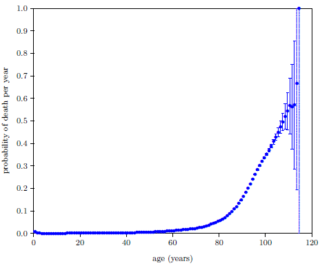The probability of death per year, P, is seen to be quite small for the first four or five decades of life, but by 80 years the probability of death per year is well above zero and bending sharply upward.

The error bars are calculated as the square root of the actual number of deaths per year divided by the number of survivors at the beginning of the year (measured from the annual birthday of the individual), starting from the actual total number of U.S. males who died in 2016. The published actuarial table specifies deaths per year from a starting population of 100,000 individuals, not the actual number of U.S. males who died in 2016. The actual number of deaths in the United States for 2016 reported by the CDC was 2,744,248.^[83] Taking half of these to be male yields an actual starting male population of 1,372,124. Thus, to get the error bars right, the actual number of deaths per year was calculated from the published table using this starting population size rather than 100,000.

The calculated error bars are too small to be seen in Figure 18.2 for most of the data points, but they become quite large as age increases beyond 100 years. These large error bars result from the relatively small numbers of survivors beyond 100 years today.

Now the Aardsma model needs to be transformed from its survival form to its probability form.

The defining differential equation for the Aardsma model has been previously specified, in Equation 4.6, as:

This can be transformed to probability of death per unit time by dividing both sides of the equation by -N.

The left side of the equation is now the probability of death per unit time. Call this simply P from now on. In practice, P is just the number of deaths in a given time interval divided by the number of survivors at the beginning of the time interval and divided by the length of the time interval. For the 2016 actuarial life table for males, P for the first year of life is just (6364 / 1,000,000 / 1 =) 0.006364, and for the second year of life it is (429 / (1,000,000 - 6364) / 1 =) 0.000432. This makes the transformed generalized Aardsma model to be:

Step 2b: Eliminate Contaminated Data Points

The next task is to select the data points to be included in the least-squares fit. The goal is to minimize the impact of age-dependent extraneous deaths on the fit.

Each data point gives a probability of death for a given age. The probability of death for a given age is the sum of the probabilities of death for numerous causes of death at that age. Potential causes of death include both congenital vitamin deficiency diseases and extraneous deaths such as murder and automobile accident. All of the data points are contaminated with extraneous deaths to some extent, but some points are much more contaminated than others. Extraneous deaths become less and less noticeable as age increases. In the first four or five decades of life, the aging diseases are not very developed, so most deaths are due to extraneous causes. But this reverses in the latter decades of life. Development of the aging diseases is then advanced, causing most deaths to be due to aging disease and causing extraneous deaths to become relatively minor.

Figure 18.3 allows the typical magnitude of extraneous deaths to be estimated.

Figure 18.3: 2016 actuarial life table data for U.S. males. Data points are plotted as blue dots. Error bars are shown as vertical blue lines through the data points. Note that the first blue dot corresponds to neonatal deaths, discussed previously.

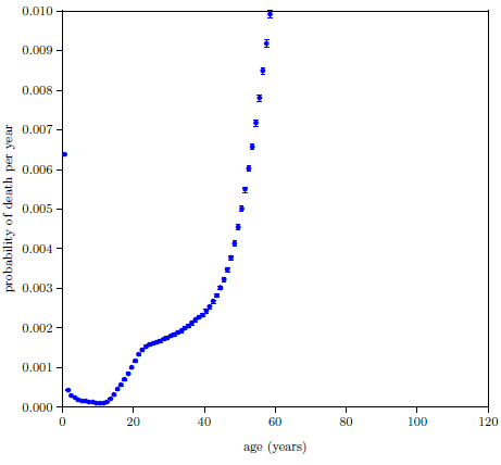It shows the 2016 actuarial life table dataset for U.S. males with the probability axis expanded by a factor of one hundred. The data have gone off scale by age 60. Aging is significantly developed by age 60, so data points up near age 60 aren't very helpful for the present purpose because they mix together both significant aging deaths and significant extraneous deaths. But below about age 40, aging is not very developed, so these ages provide a good estimate of the typical size of the probability of death due to extraneous causes. This suggests that extraneous deaths can be expected to account for a probability of death per year of say less than about 0.0025.

This means that data points having a total probability of death per year greater than 0.025 can be expected to be contaminated at less than a (0.0025/0.025×100 =) 10% level, data points having a probability of death per year greater than 0.05 can be expected to be contaminated at less than a 5% level, and data points having a probability of death per year greater than 0.25 can be expected to be contaminated at less than a 1% level.

For the 2016 dataset for males, the 10% (0.025) level corresponds to age 71, the 5% (0.05) level corresponds to age 79, and the 1% (0.25) level corresponds to age 95. Adopt the 5% level as the cutoff at this stage. That is, keep all data points from age 79 on.

Next, the fit needs some data points in the low age range. Figure 18.4 provides visual assistance with this.

Figure 18.4: 2016 actuarial life table data for U.S. males. Data points are plotted as blue dots. Error bars are shown as vertical blue lines through the data points.

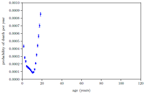It shows the 2016 actuarial life table dataset for U.S. males with the probability axis expanded by a factor of one thousand. Extraneous deaths fall off fairly rapidly from both sides to a minimum between 10 and 11 years of age. This minimum—below 1 death per 10,000 individuals per year—seems likely to be mainly due to random extraneous deaths, which are included in the model by the R parameter. So points near this minimum should not introduce any large error into the fit.

Keep the three points closest to this minimum. That is, keep the ages 9, 10, and 11 data points.

These choices retain 39 data points at this stage: the 36 data points from age 79.5 (i.e., for the time interval from 79 to 80 years of age) to the end of the dataset, plus the three data points displaying the lowest P values of the entire dataset, from ages 9.5, 10.5, and 11.5 inclusive.

Step 2c: Fit the 2016 Male Dataset

Figure 18.5 shows the fit of Equation 18.4 to the selected data points.

Figure 18.5: 2016 actuarial life table data for U.S. males. Data points are plotted as blue dots. Error bars are shown as vertical blue lines through the data points. The weighted least-squares fit of the Equation 18.4 model to selected data points is plotted as a magenta line.

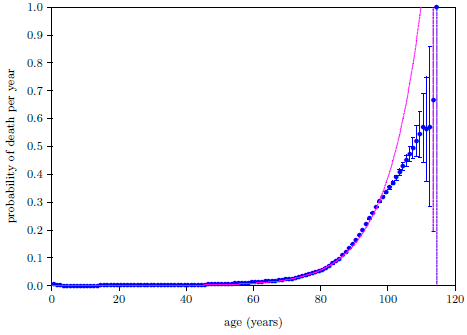This gave Χ_ν² = 54.7 with 36 degrees of freedom—still a long way from 1.5—signaling a surprisingly poor fit.

The reason for the poor fit is visually apparent from the graph. The data deviate from the expected exponential growth, shown by the magenta line, beginning somewhere after age 90.

The most obvious question to ask in such a case is whether the data can be trusted. This unexpected slowing of the rate of increase of P happens in the nineties, and not a lot of people make it to their nineties. Is it possible that the slowing is just a statistical anomaly with this particular dataset?

No, it is not possible. We are assured by the quotation from the Social Secuity Administration given previously that, for the general case, the "death rates… rise, in a roughly exponential fashion, before decelerating (or slowing their rate of increase) at the end of the life span."^[84] This plainly says that the slowing down is always seen in all datasets. The problem is clearly with the model, not with the data.

These data are insisting that the modeled aging disease does not continue to progress exponentially indefinitely as the Aardsma model assumes. Even though the modeled vitamin deficiency disease still continues to progress past age 90, its rate of progression slows down.

This is very significant. It means that the development of the modeled vitamin deficiency disease is subject to one or more limiting factors—that progression of this disease saturates (i.e., slows down and eventually ceases).

This singles out MePiA deficiency as the aging disease being modeled. While there is no obvious theoretical reason why MePA deficiency disease should ever saturate, there is an obvious reason why MePiA deficiency disease could saturate.

MePiA deficiency results in ROS damage to the mitochondria. The primary role of mitochondria is energy production for the cell. Now here is the important thing in the present context. Cells can obtain energy not only via their mitochondria but also via glycolysis. While the role of glycolysis varies by cell type, in general, mitochondria carry most of the load of energy production for the cell, with the contribution from glycolysis being minor.

The existence of these two different energy sources means that cellular energy supply will not drop to zero as, due to increasing dysfunction of ROS-damaged mitochondria, mytochondrial energy production drops to zero. Rather, cellular energy supply will drop no lower than its production via glycolysis.

Thus, the rate of increase of cellular dysfunction and death due to energy starvation, leading ultimately to whole organism dysfunction and death, will approach a constant saturation level even though mitochondrial energy supply to the cells approaches zero.

The Theory of Modern Human Aging is thus found to have an explanation for this unanticipated saturation feature of real human aging data. This is a very important result for two reasons. First, it shows that the Theory of Modern Human Aging works with real-life data, corroborating the theory. Second, it singles out MePiA deficiency disease as the aging disease responsible for saturation, which implies that the mode of action of MePiA deficiency disease is primarily energy starvation.

These fundamental concepts need to be retained and highlighted. I will do so by incorporating them at this time into the Theory of Modern Human Aging.

Theory of Modern Human Aging: Modern human aging is a congenital nutritional deficiency disease syndrome (called MHA) of two newly-discovered, closely-related vitamins: methylphosphinic acid (MePiA) and methylphosphonic acid (MePA).

Vitamin MePiA functions as an antioxidant within the mitochondria, protecting them from free radical damage due to reactive oxygen species (ROS). The fundamental cause of death resulting from vitamin MePiA deficiency is cellular energy starvation due to decreased energy output from ROS-damaged mitochondria.

Vitamin MePA functions as its own unique vitamin, separate from vitamin MePiA. It is involved in multiple biochemical pathways, similar to members of the traditional vitamins, and like them its dietary deficiency gives rise to its own unique, potentially fatal disease.

18.4.3  Step 3: Change the Model to Describe Saturation of MePiA Deficiency Disease

The mathematical model is now in need of an alteration. The description of death due to MePiA deficiency disease needs to be improved to allow for saturation.

The cause of death via MePiA deficiency disease is now taken to be energy starvation of the cells of the organism. This results from dysfunction of mitochondria due to ROS damage. So the first step is to model energy starvation due to mitochondrial dysfunction. To do this, it is necessary first to have some scheme in mind for how mitochondrial dysfunction develops with time.

Step 3a: Work Out a Dysfunction Development Scheme

I suggest that mitochondrial dysfunction develops primarily as a result of loss of vital information from the mitochondrial DNA (mtDNA) due to ROS-damage-occasioned mutations of the mtDNA.

Most DNA is in the nucleus of the cell. This is sometimes called "nDNA." But, as it turns out, mitochondria have their own relatively small amount of DNA. This is called "mtDNA." The mtDNA is vital to the functioning of the mitochondria. It provides for the synthesis of special biomolecules essential to the functioning of the mitochondria.

ROS damage to mitochondria is expected to produce genetic mutations within the mtDNA. DNA in general may be regarded as the blueprints of an organism, defining not only the organism's growth and development but also its ongoing operation and maintenance. Protecting the blueprints is necessarily of highest priority for any organism.

A house is constructed by working from a set of blueprints. The blueprints code the idea of the building. Change the blueprints, and the idea changes. A different building gets constructed. The physical building is simply the tangible expression of the idea coded by the blueprints.

Living organisms are also constructed from blueprints. While house blueprints are made of paper and ink, biological organisms' blueprints are made of DNA.

The DNA codes the idea of the organism. The fish idea is quite different from the bird idea, for example, and the DNA code for the two is quite different.

In writing, we use words and sentences to code ideas. Here is an example of an idea coded in writing using a typewriter:

The box was red.

Now here is the important point in the present context. Coded ideas are rather fragile things. Watch what happens to the idea

The box was red.

The fox was red.

Most coding errors result in something unintelligible, like this:

The gox was red.

Imagine a storybook which suffers ongoing random changes to its letters. Meaning is slowly lost. Eventually, the book has accumulated so many errors that it becomes unreadable. The original idea of the story can no longer be discerned.

For cells, coded gibberish represents erosion of the idea of the organism with concomitant loss of functionality. Cells are marvelously resourceful and able to withstand some loss of function, but the principal expectation of accumulating gibberish is eventual death of the cell. For this reason, maintaining the fidelity of its DNA code is necessarily of highest priority for any organism.

Each mitochondrion possesses multiple copies of mtDNA, all of which would be identical in a completely healthy mitochondrion. Genetic mutation of one or more copies of mtDNA within a mitochondrion produces conflicting blueprints. This is known as heteroplasmy. I propose that the loss of energy from the mitochondria is due to increasing heteroplasmy with age.

Step 3b: Model the Energy Loss

I will use a simple Gompertz function to model this energy loss with time. This models the decline in mitochondrial energy output by treating the mitochondria as classically aging entities. This seems appropriate since ROS damage to the mitochondria will be congenital and ongoing throughout life. Furthermore, a plateau phase is expected early on during which there is minimal effect on mitochondrial energy output due to ROS damage because each mitochondrion possesses multiple mtDNA copies. Early on, the mitochondrion is still able to manufacture the special biomolecules it needs to do its job by working from yet functional copies of the blueprints. Only as heteroplasmy grows large enough does supply of the special biomolecules begin to become compromised. This scheme may thus be represented by a familiar ski-slope mitochondrial energy "survival" curve, making a Gompertz function a suitable model thus:

where E_m is the time-dependent (age-dependent) energy supply from the mitochondria to the cells of the organism.

To get the total cellular energy supply to the cells, the contribution from (age-independent) glycolysis, E_g, must be added to the mitochondrial contribution. This results in a total energy supply to the cells, E, of:

Now all that is needed is an equation relating the probability of death of the organism due to energy starvation to the total energy supply.

Step 3c: Model the Probability of Death

I will take the probability of death due to energy starvation to be inversely proportional to the energy supply, normalized to zero probability of death due to energy starvation at birth (corresponding to normal, new, healthy mitochondria). This gives the probability of death due to vitamin MePiA deficiency disease, P_v1, as:

where the proportionality constant has been absorbed into the definition of E since only the form of the probability-of-death equation is of interest in the present context.

The (saturation) model is now:

Step 3d: Fit the MePiA Deficiency Disease Saturation Model to the 2016 Male Dataset

The fit of the Equation 18.8 single-disease model to the selected data points is shown in Figure 18.6. The model now has five free parameters: R, E_m0, E_g, α, and β, leaving 34 degrees of freedom. The goodness-of-fit parameter, Χ_ν², returned for this fit was 1.4, emphasizing that the saturation model is remarkably better than the non-saturation model was at describing this dataset. The fact that the fitted line visibly departs from the measured data beyond about 100 years of age shows that a single-disease model cannot properly describe the entirety of the dataset. Inclusion in the model of the second aging disease is thus seen to be mandatory.

Figure 18.6: 2016 actuarial life table data for U.S. males. Data points are plotted as blue dots. Error bars are shown as vertical blue lines through the data points. The weighted least-squares fit of the Equation 18.8 model to selected data is plotted as a magenta line.

18.4.4  Step 4: Upgrade the Model to Include MePA Deficiency Disease

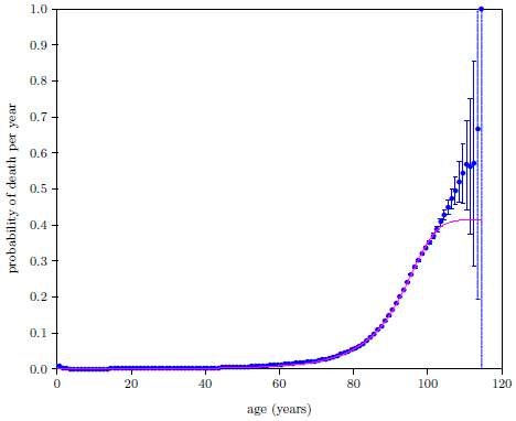MePA deficiency disease, like most aging diseases, does not saturate. It is properly described by the term from the transformed Aardsma model, Equation 18.4, containing the exponential:

Inclusion in the model of this second deficiency disease yields:

Written out explicitly, this becomes:

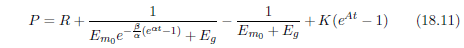
This is now a seven-parameter fit: R, E_m0, E_g, α, β, K, and A.

Figure 18.7 shows the final weighted least squares fit of the model to the 2016 actuarial life table datasets for U.S. males together with the separate contributions from the two vitamin deficiency diseases, and Figure 18.8 shows the same thing for U.S. females.

Figure 18.7: Weighted least-squares fit (magenta) of the final (Equation 18.11) model to the 2016 actuarial life table data for U.S. males. The contribution of MePA deficiency disease to the fit is shown by the black line, and the contribution of MePiA deficiency disease to the fit is shown by the orange line. Fitted parameter values and uncertainties for the graph are shown in the table.

Figure 18.8: Weighted least-squares fit (green) of the final (Equation 18.11) model to the 2016 actuarial life table data for U.S. females. The contribution of MePA deficiency disease to the fit is shown by the black line, and the contribution of MePiA deficiency disease to the fit is shown by the orange line. Fitted parameter values and uncertainties for the graph are shown in the table.

18.5  Discussion

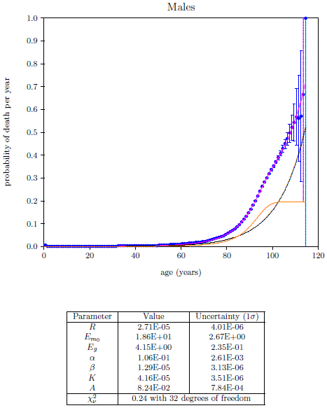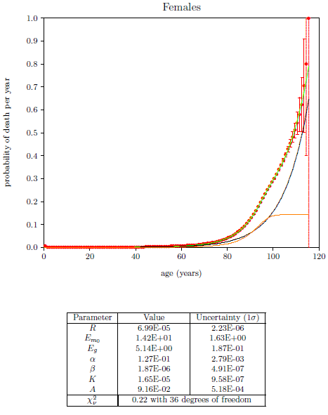Perhaps the most conspicuous observation from Figures 18.7 and 18.8 is that MePA deficiency disease dominated human mortality in the U.S. in 2016. Table 18.1 quantifies this.

Table 18.1: Numbers of deaths in 2016 resulting from MePiA and MePA deficiency diseases and other causes according to the Theory of Modern Human Aging.

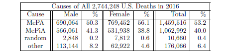Roughly 53% of total deaths from all causes in 2016 were due to MePA deficiency disease according to the model. Another 40% of total deaths from all causes in 2016 were due to MePiA deficiency disease. Thus, these two aging diseases alone accounted for over 93% of total deaths from all causes in 2016.

Of course, there is nothing particularly special about 2016. This same loss of life happens year after year. The tragedy is that it continues to happen even though it is now unnecessary. Just as scurvy can be prevented by adequate daily intake of vitamin C, MePA deficiency disease can be prevented by adequate daily intake of vitamin MePA, and MePiA deficiency disease can be prevented by adequate daily intake of MePiA. Dr. Aardsma's Anti-Aging Vitamins dietary supplement is able to eradicate MePA deficiency disease and MePiA deficiency disease just as vitamin C has eradicated scurvy, and just as vitamin B₃ (niacin) has eradicated pellagra, and just as vitamin B₁ (thiamin) has eradicated beriberi. The model finds that when this happens, some two and a half million U.S. lives—males and females of all ages—will be saved per year.

18.6  Conclusion

This study of the modern human life span data has revealed that both MePA deficiency disease and MePiA deficiency disease share significantly in modern human aging deaths so that neither may be safely ignored or negelected. It is necessary to cure both of these diseases to cure modern human aging (MHA).

Finally, we have learned that these two diseases alone fully explain MHA. Since Dr. Aardsma's Anti-Aging Vitamins dietary supplement^[86] contains both of these vitamins, it may properly be regarded as the cure for MHA.

Chapter 19

Explaining Ancient Historical Human Life Spans

The Theory of Modern Human Aging provides a full, quantitative explanation of the pattern of modern, single-year actuarial data. Can this theory also quantitatively explain the pattern of the ancient, multiple-century, biblical life span data? The present chapter shows that it can. This is accomplished by first putting the theory into mathematical form. To solve the resulting equations requires use of numerical methods on a computer. The resulting mathematical computer model is then applied to the biblical life expectancy data, revealing the match between the theory and the real-life data once again.

It is necessary to model the data quantitatively for two reasons. The first reason is to test the theory against the ancient life expectancy data. It is one thing to draft a qualitative theory of a complex process such as changing life spans. It is quite another thing to get the qualitative theory to agree quantitatively with real-life data. This will not happen by chance. Will the theory succeed with the biblical life expectancy data or be falsified by it?

The second reason is to be able to learn as much as possible about the nature of the anti-aging vitamin duo from these ancient data. For example, it is clear, as discussed in Section 8.3 and at the end of Subsection 12.1.1, that MePiA must have a long biological half-life. The need is to move beyond this qualitative observation to an objective quantitative appraisal of the biological half-life—to get the best objective, quantitative estimate possible of this and other parameters from the available data.

The biblical life expectancy data are the only data that presently exist on the effects of vitamins MePA and MePiA on human longevity. To exploit these data fully to the benefit of the planet's modern human population, a rigorous mathematical model of these data is mandatory.

While the mathematics involved in this model are not quite so challenging as those involved in the model of the previous chapter, readers beginning to feel lost or overwhelmed at any point may skip down to the Conclusion of this chapter.

19.1  The Model

The mathematical computer model was constructed using Fortran. The source listing can be found in Appendix B. The result of the model is shown in Figure 19.1. The model clearly succeeds in explaining the biblical life span data. This demonstrates both that the theory is sound and that the biblical life span data are valid historical observations.

Figure 19.1: The results of the model are shown by the red and blue lines.

19.1.1  Details

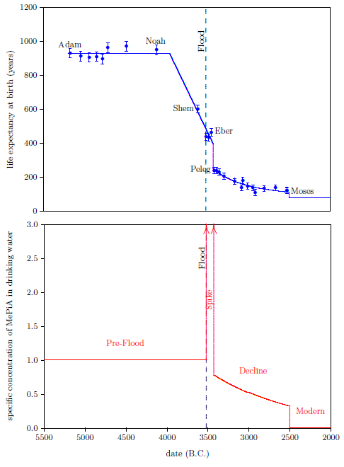The model involves two components: environmental and physiological. The environmental component yields the concentration of MePiA in drinking water. (The choice of MePiA rather then MePA will be explained below.) This is shown by the red line in the bottom graph in Figure 19.1. This is the driving function for the physiological component, which calculates the theoretical life expectancies shown as the solid blue line in the top graph.

For the sake of the model, the biblical longevity data were treated as point estimates of mean life expectancy at birth, as previously discussed. The first eight data points were simply averaged, resulting in the height of the initial horizontal blue line. These eight points were otherwise excluded from the model. The line through the remaining 18 data points results from a least-squares fit of three free (i.e., adjustable) parameters. Two free parameters were needed to describe the changing environmental abundance of MePiA, and another free parameter was needed to describe the physiological response to MePiA.

Environmental Component

The environmental component of the model was divided into the four distinct periods discussed in Chapter 9: Pre-Flood, Spike, Decline, and Modern. All drinking water concentrations of MePiA in all time periods were scaled with respect to the (unknown) concentration required for adequate daily dietary intake of this vitamin, yielding the "specific concentration of MePiA in drinking water" plotted in the bottom graph of Figure 19.1. The Pre-Flood specific concentration is unknown, but it is known to have been adequate to meet physiological requirements, so it is plotted as 1. The Spike specific concentration is also unknown, but it is known to have been much larger than the Pre-Flood specific concentration. It is plotted as a spike of indefinite height to illustrate this. These unknowns do not affect the model because any daily intake of MePiA in excess of the (unknown) adequate amount is assumed by the model not to have been retained by the body—the model treats any specific concentration in excess of 1 as being equal to 1.

The atmospheric concentration of MeP was very large during the Spike for reasons discussed at the end of Chapter 11.Just how large is unknown, but we can get a rough idea as follows. Prior to the Flood, assuming steady state conditions, the rain of phosphorus-rich detritus onto the sea floor surrounding Antarctica supplied a flux of MeP to the atmosphere, resulting in a specific concentration of MePiA in drinking water sufficient to meet physiological requirements. This MeP flux was halted when the Flood caused nearly the entire sedimentary supply of MeP to be vented to the atmosphere. The rain of phosphorus-rich detritus onto the ocean floor around Antarctica resumed after the Flood. At present, five and a half thousand years after the Flood, human longevity indicates that the specific concentration of MePiA is still effectively zero. Subtracting 1,000 years to allow for transport of MeP from the ocean floor to the atmosphere at present yields a minimum of 4,500 years' worth of pre-Flood MeP vented to the atmosphere during the Flood. Thus, the flux of MeP to the atmosphere during the year of the Flood increased by at least a factor of 4,500.

The end of the Spike interval coincides with the Eber–Peleg Drop. This drop may have happened anywhere between the third (Eber) and fourth (Peleg) data points following the Flood. The model gives a best fit when the total duration of the Spike is taken as 90 years, placing the drop in the year 3430 B.C.

The atmosphere was being provided with MeP from the oceanic reservoir during the Decline interval. The Decline interval ends with the Moses Drop in 2504 B.C., as calculated in Subsection 9.1.2. This drop signals the exhaustion of the oceanic MeP reservoir.

The existence of the Moses Drop means that the oceanic supply of MeP came to an end suddenly rather than gradually. The whole ocean slowly circulates vertically, dense (cold, saline) water formed in the north during winter sinking rapidly each year to the bottom, pushing the overlying water of the entire ocean slowly upward. The Moses Drop implies that, in the (3520 - 2504 =) 1,016 years it took Flood ocean bottom water to rise to the surface, this Flood ocean bottom water did not mix significantly with the underlying post-Flood ocean water. This, in turn, implies strong stratification between these two bodies of water, which implies that they had significantly different densities. Thus, the existence of the Moses Drop informs us that Flood ocean bottom water at the end of the Flood was significantly less dense than newly formed post-Flood ocean bottom water that began flowing down under it from the north.

This is expected. It seems inevitable that the Flood would have effectively homogenized the pre-Flood oceanic water mass. Normally, bottom water is more dense than any other ocean water because it is colder and more saline than any other ocean water. Surface waters are least dense, being warmed by sunlight. Homogenization of the pre-Flood ocean by the Flood would have produced a body of Flood ocean water having a temperature and a density intermediate between normal bottom waters and normal surface waters. Thus the density of this well-mixed body of waters from before the Flood would have differed significantly from the density of newly formed, post-Flood bottom water.

The idea that the Flood homogenized the oceans is supported by simple geometrical considerations. The average depth of the oceans is 3.8 kilometers (2.4 miles). The average travel distance for ocean water during the Flood was roughly one quarter of earth's circumference during the waxing of the Flood, then another one quarter of a circumference back again at the waning of the Flood. This is a total distance of roughly 20,000 kilometers (12,000 miles). Thus the ratio of the depth to the distance traveled is less than one five-thousandth. It seems nearly impossible to maintain density stratification in such a geometry, and it seems especially so when one considers that the flow was over uneven ocean floor and continental terrain.

The two environmental free parameters mentioned above were needed to describe the specific concentration of MePiA in drinking water during the Decline, which is modeled as a decaying exponential. Decay may have been due to internal oceanic chemical and/or biological processes consuming MeP precursor and/or to slow removal of MeP by sparging via gas bubbles rising from the ocean floor. The first free parameter sets the amplitude of the exponential, and the second free parameter sets its rate of decay.

In the Modern time period, the model takes the flux of MeP to the atmosphere to be zero. This is an approximation, but it is believed to be a very good one.

It is not likely that the Flood obliterated every last bit of natural source of atmospheric MeP. For example, Figures 12.1 and 12.2 showed that the Bering Sea enjoys high surface concentrations of nitrate and phosphate similar to ocean water surrounding Antarctica. The Flood is not expected to have significantly disturbed sea floor sediments in the northern hemisphere. Thus, it is possible that sea floor sediments in the Bering Sea are a minor source of atmospheric MeP today.

The Flood dramatically reduced the source of atmospheric trace gas MeP, perhaps by a factor of a thousand, or a factor of ten thousand, but it likely did not reduce the source of atmospheric MeP completely to zero. MeP will be present as a naturally-sourced trace gas at some tiny level, however small, in the modern atmosphere.

This implies that MePiA and MePA are yet being produced at some tiny level, however small, in the atmosphere today, and this implies that naturally-produced MePA especially, because it tends to build up in natural water bodies, may be measurable at tiny concentrations in such water bodies. Indeed, detection near 0.5 microgram MePA per liter of river water has been reported.^[87] Because MePA is a natural breakdown product of phosphonates, as previously mentioned, and because phosphonates are used widely today in industry, agriculture, and warfare, it is not clear whether this MePA is natural or anthropogenic. Nonetheless, the idea that there is no (i.e., zero) naturally produced MeP in the atmosphere today should obviously be treated as a convenient first approximation only.

But it appears to be a very good first approximation. What we know about the nature of the Flood implies that MeP must have been nearly emptied from its phosphorus-rich, anaerobic sedimentary source beds surrounding Antarctica. Meanwhile, the surface area of the Bering Sea which might still be producing MeP today is quite small relative to these southern hemisphere source beds. In addition, the global constancy of life expectancies due to MHA since the Moses Drop strongly argues for the zero-MeP approximation. For example, well water might be expected to be depleted of MePiA due to such processes as sorption of small acids by soils or its utilization by microbes as rainwater moved from the surface through the soil into the well, yet modern populations drinking water from rivers or lakes show no difference in life spans compared with populations drinking water from wells.

Physiological Component

The model treats life span as a fixed quantity (like a fixed amount of gasoline) which is used up at a time-dependent rate. When life span has been completely used up, death occurs.

Prior to the Decline, MePA and MePiA were always sufficient, so only tree-of-life nutritional deficiency disease was operative. The average life span (i.e., the life expectancy) was then 929 years, due to tree-of-life nutrient(s) being (always) zero. Thus, prior to the Decline, the rate of aging due to TOLA is treated as a constant, equal to 1/929 life span per year. When this rate of aging is summed year by year, it integrates to 1 life span after 929 years have transpired.

TOLA is still in effect today, but TOLA and MHA are two separate congenital nutritional deficiency diseases, and their rates of progression are summed separately. Whichever integrates to 1 first is the cause of death.

In the Modern time period (i.e., subsequent to the Moses Drop), male life expectancy is 76.8 years.^[88] The rate of aging due to MHA is always 1/76.8 life span per year as a result of MePA and MePiA being always zero during this period.

In the Decline time period, MHA was active, but the concentrations of MePA and MePiA in drinking water were not zero, and at least one of the concentrations of these two vitamins was inadequate to meet physiological requirements. MePA and MePiA were being supplied to the environment via the inventory of dissolved MeP gas in ocean water slowly venting to the atmosphere. Thus, the rate of MHA was changing year by year during the Decline time period.

The rate of MHA is taken by the model to be a function of the specific concentration (SC) of MePiA in drinking water as MePiA is believed to be the dominantly deficient vitamin during the Decline. SC is the ratio of the concentration of MePiA in drinking water divided by the concentration of MePiA adequate to meet the body's needs. SC is modeled as a decaying exponential:

where t_F corresponds to the end of the Flood. The oceans were homogenized by the Flood. MeP from the oceans began to decline at depth due to chemical and biological reactions and/or sparging from that point on. SC₀, λ, and t_S are all adjustable parameters of the model.

There are two known points for the rate of MHA: 1) for SC = 0 (no MePiA), the rate of MHA is 1/76.8 life span per year, and 2) for SC = 1 (adequate MePiA), the rate of MHA is 0. These two points allow a simple linear interpolation for the rate of aging due to MHA (ROA_MHA) versus SC to be specified:

The physiological free parameter in the model is the lifetime of MePiA in the body. Here again, exponential decay was assumed.

19.2  Results

19.2.1  Environmental Free Parameters

Duration of the Spike

The duration of the Spike was not a free parameter of the mathematical optimization of the goodness of fit parameter, Χ_ν², because it is a discrete, integer variable. Nonetheless, it could be optimized by giving it different values in separate runs of the computer model. When this was done, 90 years was found to be the duration yielding the best goodness of fit, as mentioned above. This implies that the large spike of MeP which the Flood released from the sediments surrounding Antarctica took 90 years to clear from the atmosphere.

Normally, MeP, which is easily oxidized, has a lifetime of only a few days at best in the atmosphere. The implication seems to be that the atmospheric chemical reactions which normally keep the atmosphere free of unwanted gases were significantly overloaded during the Spike interval. This overloading would have been contributed to by other anaerobic sea floor gases, especially methane.^[89] Thus, it appears that earth's atmosphere may have been significantly polluted globally during much of the Spike.

Amplitude of the Oceanic Reservoir

The amplitude of the oceanic reservoir free parameter is the contribution of the oceanic reservoir to the specific concentration of MePiA in drinking water (SC) in 3519 B.C., immediately following the year of the Flood. The model yields a value of 0.843±0.010 for this parameter. (All error estimates from the model are ±1σ.)

Loss of MeP Within the Oceanic Reservoir

The second environmental free parameter specifies the rate at which MeP was lost from the oceanic reservoir, either internally due to chemical and biological degradation, or directly to the atmosphere by sparging. Biological processes may have been dominant as "C-P lyase genes are abundant in marine microbes."^[90] The model yields a value of (9.34±0.12)×10^-4 per year for this parameter. This means that it took these internal processes about 740 years to deplete the flux of MeP from the oceans by a factor of two.

19.2.2  Physiological Free Parameter

Lifetime of MePiA

The model finds a lifetime for MePiA in the body of 877±111 years. The corresponding biological half-life is 608±77 years. This is an extraordinarily long biological half-life, implying specialized mechanisms for conservation of MePiA, as discussed at the end of Subsection 12.1.1.

19.3  Conclusion

It is clear, by visual inspection of Figure 19.1, that the fit of the model to the data is quite good. The goodness-of-fit parameter, Χ_ν², for the least-squares fit was 1.18 with 15 degrees of freedom. The model has succeeded in capturing the panoramic essence of the biblical life expectancy data and in quantifying its free parameters.

The model's greatest deficiency appears to be that it finds a life expectancy which seems certainly too low just prior to the Moses Drop. The blue dot labeled "Moses" is actually two data points close together, one for Moses and the other for Aaron. While the actual life spans in these two instances were 120 and 123 years respectively, the model predicts a life expectancy of 107 and 108 years for these two individuals. This results, not from statistical scatter, but from over-simplification of this part of the model.

Specifically, in real life there would have been an "echo" of the Spike during the lifetimes of Moses and Aaron which is not included in the model. This "echo" results from the fact that during the Spike, newly formed ocean bottom water would be enriched in dissolved MeP precursor gas relative to prior and subsequent years. Recall that ocean bottom water is formed from dense (cold, saline) northern surface water sinking each winter. This water would be in contact with the atmosphere prior to sinking. Since the atmosphere contained an unusually high concentration of MeP during the Spike, bottom water originating during the Spike would also contain an unusually high concentration of MeP. This is not included in the model. The model treats the Decline phase as a simple exponential decay. To be more realistic, the Decline would need to be modeled as an exponential decay plus a "hill" at the end of the Decline. (This "hill" would likely be a Gaussian, resulting from diffusion of the elevated MeP during the roughly one thousand years needed for the Spike-formed bottom water to rise to the surface.) Such fine detail has been neglected in the current model to keep things as simple as possible at this stage.

The success of the model drives home the conclusion that the biblical life expectancy data cannot be mythological or otherwise fabricated. What did the ancient author of Genesis understand about methylphosphine (MeP), about its reactions with oxidants in the atmosphere yielding methylphosphinic acid (MePiA), about Antarctica, about upwelling phosphate and nitrate in the southern oceans, about vitamins and vitamin deficiency diseases, about anaerobic digestion within sea floor sediments, about the baring of southern ocean floors during the Flood? Yet, all of these things and more must be properly understood to explain the pattern of these biblical life expectancy data points. The only reasonable explanation of the amenability of these ancient biblical life expectancy data to quantitative, scientifically rigorous analysis is that they are accurately recorded, real-life observations.

Conversely, the goodness of the fit to these data validates the model and its theoretical underpinnings.

Chapter 20

Potential Longevity Today

At present, we live in a world dominated by MHA disease. Progression of MHA is nearly zero in infants and nearly terminal in centenarians. But MHA is now beginning to be driven back. Eventually, it will be eradicated from our planet.

When MHA has been eradicated from the global population by adequate daily intake of MePiA and MePA, then human longevity will revert back to pre-Flood longevity, exemplified by the 929-year life expectancy at birth enjoyed by pre-Flood males.

This will clearly be an enormous improvement on modern human longevity, but notice that the 929-year average life span of pre-Flood males was not a limiting life span any more than the current 77-year average life span of modern males is a limiting life span. According to the ancient biblical record, the 929-year, pre-Flood life expectancy was a result of TOLA disease. This disease was imposed, not natural. Thus, humans were not designed to die of aging, and there appears to be no limiting life span for humans. This implies that conquest of TOLA will pose the final frontier for research into human aging disease, after which potential human longevity will become infinite once again.

This is not to say that eradication of the final aging disease will grant immortality, for it most certainly will do no such thing. Eradication of aging diseases does not stop speeding bullets, for example. Eradication of aging merely removes the congenital diseases of aging as particular causes of death.

While we wait for MHA to be eradicated, what extension of life span might MHA-diseased individuals anticipate once they have begun to take Dr. Aardsma's Anti-Aging Vitamins?

20.1  Method

There are no experimental data from humans on this question at present, nor are there likely to be any experimental data on it any time soon. Experimental evidence for life lengthening due to the anti-aging vitamins has only recently been obtained from the experiments with mice discussed in previous chapters. Mice experiments typically take three years to complete. Because humans live about 30 times longer than mice at present, experimental evidence for life lengthening in humans seems likely to be decades away. At present, to predict the probable effect of the anti-aging vitamins, MePiA and MePA, on human life spans, it is necessary to rely on theory.

20.1.1  Life Expectancy

No one can say with certainty how long anybody will live, of course, but on average at present, in our MHA-diseased population, we expect infants to enjoy a life span of something like 70 or 80 years, and we expect 40-year-olds to live something like another 30 or 40 years. Because discrete, individual life spans cannot be predicted, it is necessary to talk about the average life span of a group of individuals. The average life span remaining for a group of same-age individuals is called their "life expectancy." The life expectancy today for infants will be something like 70 or 80 years, and the life expectancy for 40-year-olds will be something like 30 or 40 years.

Questions about life expectancy are routinely answered today using actuarial life tables. An actuarial life table shows the probability of dying within the year from one birthday to the next. The present analysis uses the same (2016) Social Security Administration actuarial life table which was used in the modeling study of modern human life spans in Chapter 18.^[91] Both the number of survivors and the life expectancy versus age are included in the 2016 SSA table. In the present chapter, the 2016 table is treated as representative of what is normal in the case of well-cared-for humans whose diets completely lack the anti-aging vitamins from birth on.

Figure 20.1 shows the SSA table's life expectancies versus age graphically.

Figure 20.1: Life expectancy for modern U.S. males (blue) and females (magenta) not taking the anti-aging vitamins.

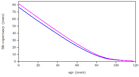Life expectancies for males and females are graphed separately, reflecting their separation in the actuarial table. This graph shows that newborn male babies have a life expectancy of 76 years, and newborn female babies have a life expectancy of 81 years; 40-year-old males have a life expectancy of 38.6 years, and females 42.5 years; and 80-year-old males have a life expectancy of 8.3 years, and females 9.7 years. What happens to these life expectancies when an individual converts from a diet devoid of the anti-aging vitamins to a diet containing adequate anti-aging vitamins?

20.1.2  Computer Program

To answer this question quantitatively, it was necessary to use numerical methods via a computer program once again (Appendix C). The program calculated the new life expectancies for males and females first beginning to take the anti-aging vitamins at some age between birth and 113 years.

Physiological Agedness

To understand how the computer algorithm works, it is first necessary to understand the idea of physiological agedness.

Calendar age is a count of the number of calendar years which have passed since a person was born. Physiological age is a measure of the physiological progression from birth to "old age" of a person's body. We are accustomed to equating these two at present because the two start out together at zero. Physical growth toward maturity then progresses at a roughly equal rate in all individuals, making it possible to guess a young person's calendar age fairly accurately based upon his degree of physical maturity. Meanwhile, at the same time as growth toward maturity has been happening, the aging diseases have been progressing, making it possible to guess an adult's calendar age fairly accurately based upon the extent to which his aging diseases have progressed.

While it is now necessary to break the careless habit of equating physiological age with calendar age, this habit provides a simple and convenient scale for discussing how youthful or otherwise a person's body appears to be. It is immediately clear what is meant if one says at present that a person looks to be one year old, for example. It is clear that one means that physical development toward maturity has just gotten started. It is also immediately clear what is meant if one says at present that a person looks to be 100 years old. It is clear that one means that physiological agedness, due to the aging diseases, has come very nearly to a terminal condition. It would also be clear what was meant should one say at present that a pre-Flood individual having a calendar age of 700 years had a physiological agedness of 30 years. It would be clear that this meant that a 700-year-old person back then had a physical body typical of a 30-year-old today.

The physiological agedness scale is defined to be a measure of the physiological progression of the human body from cradle to grave, conveniently calibrated by our everyday experience at present.

Age of Terminal Maturity

Related to the concept of physiological agedness is the idea of terminal maturity, when physical development toward adulthood ceases. The possible range for terminal maturity today seems to extend from the early twenties to the early forties. The computer algorithm adopts 34 years as the calendar age of terminal maturity for modern humans.

The Computer Algorithm

The computer program begins by subtracting both the probability of dying due to MePA deficiency disease and the probability of dying due to MePiA deficiency disease from the SSA table's year by year probability-of-death data. It does this using the fitted curves for these diseases found by the modeling study of the 2016 actuarial life table data in Chapter 18 and shown in Figures 18.7 and 18.8. The residual SSA data then gives the probability of dying due to extraneous causes versus the individual's physiological age. Consider the example of a modern, 40-year-old male beginning to take the vitamins. His calendar age and his physiological age start out both together at 40 years. After he has taken the vitamins for one year, his calendar age has increased 1 year, making him 41 years old. Meanwhile, because of the vitamins, his body has begun to heal of MHA. What does this do to the man's physiological age?

The program treats MePA deficiency disease like scurvy. Scurvy is healed very rapidly by adequate dietary intake of vitamin C. The program treats MePA deficiency disease as being instantaneously cured as soon as dietary supplementation with Dr. Aardsma's Anti-Aging Vitamins has begun. This is an approximation, knowingly a little optimistic, but it is believed to be reasonably realistic based upon presently available data. If MePA deficiency were the only aging disease, then this approximation would amount to setting the 40-year-old man's physiological age back to 34 years, the assumed age of terminal maturity. His probability of dying in his fortieth year would then be just the probability of dying due to extraneous causes for a 34-year-old male. Unfortunately, MePA deficiency is not the only aging disease. MePiA deficiency must also be reckoned with.

The healing of the mess made by MePiA deficiency disease, with its consequent energy starvation of cells, is a more complex matter. Once adequate daily intake of MePiA has begun, further ROS damage to mitochondria is greatly attenuated. The program approximates this, somewhat optimistically again, by reducing further ROS damage immediately to zero. This treats MePiA deficiency disease as immediately cured, which seems a reasonable approximation because there is no longer any deficiency of MePiA and further wildfire ROS damage has been halted. MHA has been cured by beginning to take the anti-aging vitamins, but full health has not yet been restored. Stopping further wildfire ROS damage has not erased the damage already done to the mitochondria.

Present theory says that it is mutation of the mtDNA due to ROS damage which is responsible for declining mitochondrial energy production. Individual copies of the mtDNA have been mutated in divergent ways, seeding heteroplasmy throughout the organism. This sort of heteroplasmy is called "microheteroplasmy." Microheteroplasmy is the damage already done.

Microheteroplasmy is not aging, and it is not an aging disease. It is, like cancer, an aging-related disease. It is its own disease, induced by the aging disease called MePiA deficiency disease. Curing aging does not automatically cure all aging-related diseases. Curing MHA does not automatically cure microheteroplasmy.

The damage already done—microheteroplasmy—represents not simply harm to some biomolecule which might easily be repaired, but rather a loss of information from the mitochondrial blueprints regarding what the biomolecules needed by the organism are meant to look like. Restoration of this lost information is a difficult problem for the organism to solve at the biomolecular level. The mitochondrion does not "know" what undamaged mtDNA looks like. The mitochondrion possesses no indelible mtDNA copy which can be referenced in order to distinguish between pristine mtDNA and mutated mtDNA. The mitochondrion is merely a mindless machine, pumping out whatever biomolecules its multiple mtDNA copies—pristine or otherwise—specify. It appears that the mitochondrion has no way of fixing itself—no way of restoring its lost information.

It thus appears that damaged mitochondria stay damaged. But this is not the end of the story. There still seems to be a possibility of at least some degree of healing.

Theoretically, it seems possible for the organism's cells to discriminate against mitochondria that are less efficient because they have been damaged, replacing them with new copies of mitochondria that are more efficient because they are less damaged. This does not immediately restore pristine mitochondria, but it does begin to clean up the microheteroplasmy mess.

Theoretically, this can eventually restore pristine mitochondria. In the process of generating new mitochondria, by fission of a less damaged mitochondrion, mtDNA copies from the parent mitochondrion would be expected to be randomly apportioned between the two offspring mitochondria. This would result in offspring mitochondria with differing energy-production efficiencies. If, for example, one offspring mitochondrion happened to get all of the best-preserved mtDNA copies from the parent, while the other got all the most-damaged copies, this would allow further refining of the mtDNA via further discrimination against the less-efficient offspring mitochondrion.

Even if the body is able to do this, it is expected to be a very slow process, lasting decades. The program here adopts what is thought to be a worst-case scenario, setting the rate of healing of microheteroplasmy to zero. This means that the program assumes that the individual is stuck from then on with whatever probability of dying per year due to energy starvation that individual had when supplementation with Dr. Aardsma's Anti-Aging Vitamins was started.

Thus, rather than resetting the 40-year-old man's physiological age back to 34 and leaving it there, the program sets the 40-year-old man's physiological age to 40 and leaves it there. This choice is expected to yield a result which somewhat underestimates the potential longevity benefit from adequate intake of the anti-aging vitamins, but it seems the least error-prone choice based upon the state of knowledge at present.

Summarizing, after one year of supplementation, the 40-year-old man has become 41 years old in calendar years but his physiological age has remained at 40.

This neglects the possibility that he may not have lived to his 41st birthday, an oversight which will be corrected shortly. Assuming he has survived to age 41, it is easy to calculate what happens in his 42nd year. His calendar age advances to 42, and his physiological age remains at 40 years.

The program carries on in this way (albeit at higher computational precision and with smaller time steps) year by year, advancing the man's calendar age and maintaining his physiological age where it was when he started supplementing with the anti-aging vitamins. Now consider the possibility that the 40-year-old man died prior to his 41st birthday. This possibility is related to the probability of death per year for 40-year-old-men. This probability is made up of the probability of dying due to the aging diseases between age 40 and 41, plus the probability of dying due to other causes such as car accidents. For individuals not supplementing with the anti-aging vitamins, the (raw) SSA actuarial life table informs us that this probability is 0.00242. This means that out of 100,000 anti-aging-vitamins-deficient men turning 40 years old, 242 die in their 41st year for one reason or another: heart attack, brain aneurysm rupture, car accident, violent crime, etc. But the 40-year-old man in our example is not anti-aging-vitamins deficient. The program uses the residual SSA data to look up the probability of death in the next year from extraneous causes of a 40-year-old man. It then adds to this the amount of energy-starvation (i.e., damaged mitochondria) probability of death per year for a 40-year-old man. Finally, it adds to this the probability of dying of TOLA. This will be essentially zero in the early centuries but will dominate the calculation out past 800 years of age. The least-squares fit to the pre-Flood male data shown in Figure 6.2 is used to calculate the contribution TOLA makes year by year to the probability of death per year. This sum of extraneous, damaged mitochondria, and TOLA contributions gives the appropriate probability of death for the anti-aging-vitamins-supplementing 40-year-old man. The program uses this probability as part of its calculation of the new life expectancy. It starts with 100,000 men of age 40 and keeps a total of how many survive year by year of the calculation. When none (i.e., less than 0.5) remain, it stops the calculation and calculates the new life expectancy value for age 40 males.

That explains most of what the computer program does. Only two further details need to be mentioned. First, notice that the probability of death due to extraneous causes for our example male in his 42nd year is not the value found in the residual SSA actuarial table data for a 41-year-old male. Rather, it is the value one gets for a 40-year-old male. It is the physiological age which must be used in the 2016 actuarial life table for the calculation, not the calendar age. The program is using the SSA actuarial table to learn the probability of death due to extraneous causes, and this probability is related to physiological age, not calendar age.

Second, notice that there are two cases to deal with:

1. For individuals beginning supplementation after calendar age 34, the program holds their physiological age at their starting age, as described above, for all subsequent calendar years.
2. For individuals beginning supplementation before calendar age 34, the program tracks their physiological age forward to physiological age 34, at one physiological year per calendar year, then holds them there for all subsequent calendar years.

20.2  Results

The new life expectancies, calculated by the computer program, are shown in the "LE AAV" column of Table 20.1. The "LE SSA" column shows the life expectancies from the 2016 actuarial table, which are normal to MHA-diseased individuals today.

Table 20.1: Life expectancy increase factor versus age of starting dietary supplementation with adequate levels of vitamins MePiA and MePA for ages 1 to 113. The "age" column specifies the age when supplementation begins. LE SSA is the life expectancy of modern individuals of specified age not supplementing their diets with either MePiA or MePA. It is taken from the Social Security Administration's 2016 actuarial life table. LE AAV is the life expectancy of modern individuals supplementing their diets with adequate intakes of both MePiA and MePA. It is calculated by the computer program discussed in this chapter. The column headed "factor" shows LE AAV divided by LE SSA for the chosen age row. This is the life expectancy increase factor.

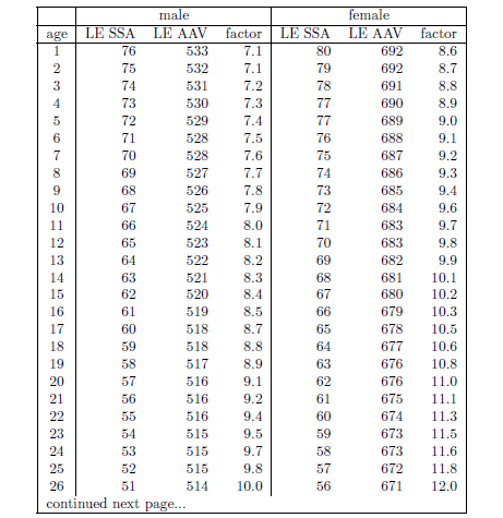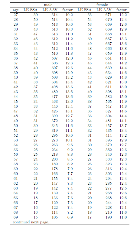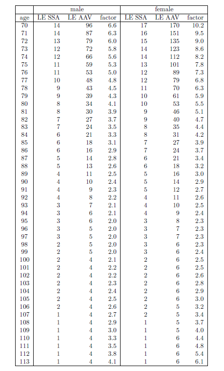Returning to the teaching example of the male beginning to supplement with the anti-aging vitamins at 40 years of age, the table shows that his life expectancy at age 40 jumps from the SSA actuarial table value of 39 years (giving a total life span expectancy of 79 years) to 508 years (giving a total life span expectancy of 548 years). For a female beginning to supplement with the anti-aging vitamins at 40 years of age, the table shows that her life expectancy at age 40 jumps from the SSA actuarial table value of 43 years (giving a total life span expectancy of 83 years) to 629 years (giving a total life span expectancy of 669 years).

As a further teaching example, consider an elderly male beginning to supplement with the anti-aging vitamins at 90 years of age. The table shows that his life expectancy at age 90 jumps from the SSA actuarial table value of 4 years (giving a total life span expectancy of 94 years) to 10 years (giving a total life span expectancy of 100 years).

20.3  Discussion

For much of the table, the new life expectancies for females come out significantly larger than the new life expectancies for males. This happens because of the large difference in the probabilities of extraneous deaths for young adult males and females. For example, at age 34 years, the extraneous death probability for females is 0.00077 per year while for males it is double at 0.00156 per year. The three leading causes of death in this age group today are unintentional injury, suicide, and homicide.^[92] The leading causes of unintentional injury death are unintentional poisoning (0.00019), dominated by drug abuse overdose, followed by motor vehicle traffic deaths (0.00012), no doubt dominated by alcohol and drug abuse, and unintentional fall deaths (0.00011).^[93] The fact that young males tend to take more unnecessary risks than young females is clearly reflected in these probability-of-death numbers.

This emphasizes that one's life expectancy, once aging deaths have been minimized, is strongly influenced by one's lifestyle choices. This is further illustrated by the fact that pre-Flood males appear to have had life expectancies at birth near 900 years, significantly greater than the roughly 530 years calculated by the computer program for modern males. This results from lifestyle differences. Pre-Flood males did not do drugs and did not drive automobiles, for example. The computer program makes no allowance for how one chooses to live. Its analysis is based entirely upon national averages for the year 2016. Table 20.1 should be utilized with this in mind. One can do better on average than the calculated "LE AAV" life expectancies if one chooses to live in less risky ways.

Another thing to bear in mind is that the nature of life expectancy itself has changed. Its definition has not changed, of course. It is still the average life span for a same-age group of individuals. But the shape of the survival curve for such a group changes dramatically once the effects of MHA have been minimized. When MHA is dominant, as it is today, life expectancy means the age at which just about everybody dies. When MHA has been minimized by supplementing with the anti-aging vitamins, the meaning changes, as Figure 20.2 illustrates.

Figure 20.2: Survival curves for U.S. females supplementing with the anti-aging vitamins (green) and not supplementing with the anti-aging vitamins (magenta). Dashed lines show the respective life expectancies at birth.

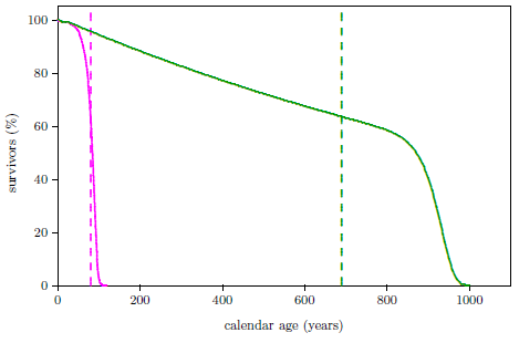The dashed vertical lines show the respective life expectancies at birth. The dashed magenta line does, indeed, correspond to when just about everybody dies, but the dashed green line most certainly does not. Few females having an adequate intake of the anti-aging vitamins from birth on, shown by the solid green line, die each year near the dashed vertical green line. The percentage of survivors declines only slowly in that region. The death rate is most rapid much later on, in the interval between about 850 and 970 years when TOLA is killing everybody off. The reason everybody dies at nearly the same time when MHA is dominant is that MHA kills everybody off in such a short span of calendar years—before most have reached even 100 years of age—that the effect of extraneous deaths is cut short and thereby minimized.

Figure 20.2 also illustrates the very long life spans which are possible once MHA has been removed. Such a world may seem impossible or unbelievable, but logic and science insist on it. Because MHA has been taking its toll on humans for thousands of years, we have grown up assuming that a 70- or 80-year life span is normal for humans. But we are entirely mistaken in this assumption. We have grown up in abnormal times with abnormally shortened human life spans relative to the totality of human history. Earth's oldest written history, found in the biblical book of Genesis, records human life spans of nearly 1,000 years prior to Noah's Flood. These ancient observational data of long human life spans are every bit as meaningful as our modern observational data of short human life spans, and they immediately teach us that it is wrong to assume that our modern times are normal. Wake up, planet Earth!

To be perfectly clear, these results, with individuals living in excess of 900 years, though calculated from theory, apply in the real world today, and they apply to ordinary people today having sufficient common sense to protect themselves from fatal diseases, including specifically MHA disease.

What do 700- or 800-year-old people look like? Do they look very, very old? No. The "old" look is purely a consequence of MHA. Individuals living to 700 or 800 years free of MHA look like mature, youthful adults.

How do 700- or 800-year-old people die? They die from all the sorts of things not related to MHA which kill normal mature youthful adults today: car accidents, homicides, suicides, lightning strikes, drownings, infections, natural catastrophes, wars, snake bites, etc.

Finally, Figure 20.2 illustrates that the modern time limit on life vanishes once adequate intake of the anti-aging vitamins has become the norm, being replaced by a ten times longer time limit on life. Because aging diseases progress exponentially, they set an artificial limit on life spans. Today, if you do not die due to some extraneous cause, then you can absolutely count on MHA killing you, in the absence of the anti-aging vitamins, before you have lived even 125 years. But once MHA is removed by lifelong adequate intake of vitamins MePiA and MePA, one does not run out of time by 125 years. Rather, one lives hundreds of years in a mature, youthful adult state, until TOLA takes over, imposing a new artificial limit on human life spans out near 930 years.

20.4  Conclusion

The foregoing numerical results of the computer calculation should not be treated as highly precise certainties. They are not that. They are approximations showing likelihood, not knowns showing certainties. They entail several assumptions and approximations, as discussed, which cannot be guaranteed. Nonetheless, what the computer calculation communicates loudly and clearly is that the advent of the discovery of the anti-aging vitamins has opened a whole new era for the human species. It makes unquestionably clear the fact that the seemingly refractory "threescore years and ten; and if by reason of strength… fourscore years"^[94] time limit on life, which has dominated all of humanity for some four and a half thousand years, has been lifted at last.

The results of the computer calculation, displayed in Table 20.1, reveal a world in the early stage of a dramatic transition. The transition is away from the dominance of the severely life-shortening MHA diseases to a world free of them. Ultimately, life spans measured in multiple centuries will be the normal experience of humanity. The prophet Isaiah, foreseeing this day nearly three thousand years ago, with poetic aptness put it this way:^[95]

For the youth will die at the age of one hundred
And the one who does not reach the age of one hundred
Shall be thought accursed.

Chapter 21

How to Maximize Your Health and Longevity Starting Now

Figure 21.1 is possibly the most succinct way of showing the benefit to health and longevity of beginning lifelong supplementation with the anti-aging vitamins at any age.

Figure 21.1: Life expectancy increase factor for U.S. males (blue) and females (magenta) starting to take the anti-aging vitamins.

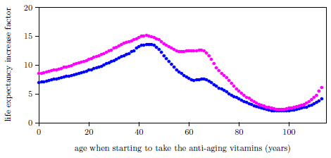Its graph does this by plotting the "factor" columns from Table 20.1. Because longevity is so intimately dependent on health, this graph may be interpreted as indicating benefit to health as well. It shows that a male who starts lifelong supplementation at age 40 will increase his life expectancy by a factor of 13.2, and a female who starts lifelong supplementation at age 40 will increase her life expectancy by a factor of 14.8. While many would give almost anything in exchange for even just one more year of life, here is opportunity to be given more than another 10 remaining lifetimes.

Notice that there are no losers with this graph. Both males and females, regardless of their age when they begin supplementation with the anti-aging vitamins, increase their life expectancies. The smallest increase displayed by this graph is a factor of 2.3 (for males aged 95–98 years).

21.1  Rule 1

Figure 21.2, a graph of the life expectancy columns from Table 20.1, shows that, for individuals supplementing with the anti-aging vitamins, life expectancy declines with increasing initial supplementation age. This means that the longer one waits to begin dietary supplementation with the anti-aging vitamins, the greater the loss to one's health and longevity.

Figure 21.2: Life expectancies for U.S. males (blue) and females (magenta) starting to take the anti-aging vitamins (dots) and not starting to take the anti-aging vitamins (solid lines).

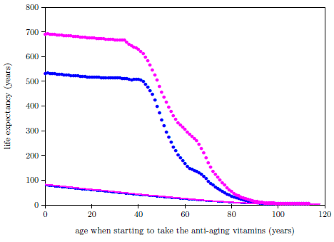This observation leads immediately to a most important point of strategy for personal use of the vitamins. I will call this point of strategy Rule 1.

Rule 1: Whatever your age, if you are not presently supplementing your diet with daily intake of the anti-aging vitamins, begin to do so without delay.

The health and longevity cost of breaking this rule can be very large. Consider, for example, a female who is first introduced to the anti-aging vitamins at age 50. Unfortunately, life has made her a bit cynical. She thinks "snake-oil salesman" to herself, and turns a deaf ear. When she reaches age 60, she changes her mind. Her hair has gone white, and her arthritis takes the joy out of life much of the time. Her friend, who started on the anti-aging vitamins a long time ago, has no arthritis and is simply more healthy and vibrant. She finally decides to start taking the anti-aging vitamins.

Had she started taking the anti-aging vitamins at age 50, her life expectancy would have been 457 years. At age 60, it has declined to 305 years. Of the 152-year difference, she has lived 10 years and lost 142 years. She has managed to squander 142 years of life expectancy—more than an entire lifetime, in modern human aging terms—in just 10 years.

It might be supposed that, nonetheless, this is not too bad—she still has 305 years of life expectancy remaining. But this is wrong-headed entirely. She now has a 60-year-old body to contend with. If she had begun taking the vitamins 10 years earlier, her aging diseases would not have progressed another 10 years. Having thus progressed, her remaining years may now be far fewer than the 305 years of remaining life expectancy suggests. The incidence of cancer is strongly correlated with physiological age. Imagine that her body had developed a cancerous cell in her 59th year which, had she begun taking the anti-aging vitamins at age 50, would not have arisen. Imagine that the cancerous cell has a doubling time of one year. Twenty years later, in her 80th year, this single cell has multiplied and become a pea-sized tumor. Her body has no natural defense against this particular cancer. Her only hope is removal of the tumor. This, of course, requires that the tumor be somehow detected. The longer it goes undetected, the greater the probability that it will metastasize, at which point removal of the tumor will do little good. Meanwhile, all of this might have been so easily avoided.

The aging diseases are not to be toyed with at any age. Wisdom calls for deliberate action against them at one's earliest opportunity.

21.2  Rule 2

There is only one other major point of strategy. I will call it Rule 2.

Rule 2: Take the anti-aging vitamins without fail every day.

The only reason Rule 2 needs to be explicitly stated and emphasized is that it is easy to get off track with the anti-aging vitamins. Healing of MePA deficiency disease is fairly rapid, resulting in obvious health improvements for many users of Dr. Aardsma's Anti-Aging Vitamins early on after they start taking the anti-aging vitamins, especially for older users. But healing of damaged mitochondria and the energy starvation of cells this damage produces is slow at best. This means that one is not likely to notice much improvement, especially after initial gains in health due to the healing of MePA deficiency disease have become the new norm. In fact, it is most likely that the microheteroplasmy mess made by wildfire ROS damage prior to beginning to take the anti-aging vitamins will result in some slow yet noticeable progression of typical "aging" symptoms. This makes it all too easy to fall prey to the feeling that the anti-aging vitamins aren't doing anything for you anymore, so you stop taking them. One must not give way to such impulses. Be assured that the anti-aging vitamins have cured your former MHA disease, and that they are actively keeping it from recurring as long as you keep taking them. Understand that the outworkings of microheteroplasmy and other aging-related diseases cannot be stopped in an instant. The return to full health is likely to be long, precarious, and discouraging, especially for older users. But to stop taking the anti-aging vitamins is exactly the wrong thing to do.

Think about it. Seriously now, would you intentionally eliminate any other vitamin from your diet?

People who unwittingly eliminated vitamin C from their diet (mostly long-ago sailors on long voyages failing to get fresh fruits and vegetables) soon became diseased with scurvy, suffering horribly from bone and muscle pain, easy bruising and bleeding, gum disease, depression, and anemia for weeks or months before succumbing to this ancient dread disease. Nobody ever intentionally eliminated vitamin C from his diet. Nobody wants scurvy.

People who unwittingly eliminated vitamin B₃ (niacin) from their diet (thousands of Southerners in the 1920's, eating inexpensive milled Midwestern corn so they could convert more of their land to cotton)^[96] soon became diseased with what is called pellagra, suffering horribly from dementia, diarrhea, and dermatitis for weeks or months before succumbing to this relatively modern dread disease. Nobody ever intentionally eliminated vitamin B₃ from his diet. Nobody wants pellagra.

People who unwittingly eliminated vitamin B₁ (thiamine) from their diet (by eating mostly polished, white rice) soon became diseased with what is called beriberi, suffering horribly from loss of appetite, irritability, mental confusion, peripheral neuropathy, swollen hands and feet, and chest pains from a malfunctioning heart for weeks or months before succumbing to this old-time dread disease. Nobody ever intentionally eliminated vitamin B₁ from his diet. Nobody wants beriberi.

Put your intellect, not your feelings, in charge. The aging diseases are insidious and deadly. You must never let down your guard against them. Treat them as deadly enemies, for they are deadly enemies.

21.3  Conclusion

Many foods and drinks are fortified with the traditional vitamins today, making it difficult not to get an adequate daily intake of these vitamins. It is to be hoped that this will eventually be the case with the anti-aging vitamins as well—that governments will come up to speed with the anti-aging vitamins and put measures in place to make it difficult for citizens not to get an adequate daily intake of them. But history shows that governments generally have a pretty poor track record with this sort of thing. In the meantime, you must look after yourself. This is not hard to do. Simply follow Rule 1 and Rule 2:

Rule 1: Whatever your age, if you are not presently supplementing your diet with daily intake of the anti-aging vitamins, begin to do so without delay.

Rule 2: Take the anti-aging vitamins without fail every day.

Dr. Aardsma's Anti-Aging Vitamins dietary supplement^[97] has been deliberately designed to make it easy for you to follow these two rules.

Appendices

Appendix A

PODfit10.F95

The program listing below shows a program I wrote and modified over several years to carry out least-squares fits of survival curve data from my lab and general research. It, or a similar predecessor, has been used to perform the least-squares fits shown in the figures in this book.

The code is in free-format Fortran 95. It was compiled as a 64-bit executable using GNU Fortran 6.1.0 via Simply Fortran by Approximatrix. The executable was run in a Windows 10 Command Prompt window on a PC having an Intel Pentium G3258 CPU.

program PODfit10
! Graphics may be displayed using a spreadsheet.
! This may be run in the SF Console or in a DOS command prompt window.
! t2 and t3 must always be set to something; to get them out of the fit, set them above the range of interest (e.g., t2 = t3 = 200.0)
!
dimension x(1000), y(1000), sigmay(1000), a(19), sigmaa(19), yfit(1000), t(1000), d(1000), t_datapoint(1000), d_datapoint(1000), include_pt(1000), chi2(1000)
CHARACTER (LEN=60):: filename1, filename2
!——————————————
print *
print *, "***Now running PODfit10.f90.***"
print *
print *, "INSTRUCTIONS (printed with every run):"
print *, "The fitting function is:"
print *, " P = R + C*exp(-E*t) + A0*[exp(E0*t)-1] + A1*[exp(E1*t)-1] + Poly + Sat for t <= t2"
print *, " P = R + C*exp(-E*t) + A0*[exp(E0*t)-1] + A1*[exp(E1*t)-1] +
A2*[exp(E2*(t-t2))-1] + Poly + Sat for t2 < t <= t3"
print *, " P = R + C*exp(-E*t) + A0*[exp(E0*t)-1] + A1*[exp(E1*t)-1] +
A2*exp(E2*(t3-t2))*{1+E2/E3[1-exp(-E3(t-t3)]} + Poly + Sat for t > t3"
print *, " where P is the probability of death per unit time, and"
print *, " where Poly approximates time-dependent extraneous deaths as follows:"
print *, "Poly = C0 + C1 * t + C2 * t^2 for t < 20"
print *, " and where Sat approximates saturating MePiA-deficiency-disease deaths as follows:"
print *, "Sat = 1.0/[Em0*exp(-(beta/alpha)*(exp(alpha*t)-1)) + Eg] - 1.0/[Em0 + Eg]"
print *, "This is random deaths plus congenital (early childhood) deaths plus aging disease 0 deaths plus aging disease 1 deaths plus aging disease 2 deaths with generic saturation,"
print *, "plus a 2nd order polynomial to describe time-dependent extraneous deaths for t < 20 years plus saturating MePiA deficiency disease deaths."
print *, "1. Set up your input file, named as you please (e.g., example.txt), stored in the same folder as this program."
print *, "The program needs starting values for parameters R, C, E, A0, E0, C0, C1, C2, A1, E1, A2, E2, t2, E3, t3, Eg, Em0, beta, and alpha."
print *, "It then adjusts the free parameters to get the best least-squares fit to your data."
print *, "The program is meant to be used side-by-side with a spreadsheet program, which does all the graphics."
print *, "Use the spreadsheet also to find (visually, graphically) reasonable starting values for the model parameters."
print *, "Put the starting value for R on line 1 of your input file followed by 1 if R is a free parameter or 0 if it is a fixed parameter (e.g., 0.0 1)."
print *, "Put the starting value for C on line 2 of your input file followed by 1 if C is a free parameter or 0 if it is a fixed parameter (e.g., 0.0 0)."
print *, "Put the starting value for E on line 3 of your input file followed by 1 if E is a free parameter or 0 if it is a fixed parameter (e.g., 0.0 0)."
print *, "Put the starting value for A0 on line 4 of your input file followed by 1 if A0 is a free parameter or 0 if it is a fixed parameter (e.g., 0.000006 1)."
print *, "Put the starting value for E0 on line 5 of your input file followed by 1 if E0 is a free parameter or 0 if it is a fixed parameter (e.g., 0.1 1)."
print *, "Put the starting value for C0 on line 6 of your input file followed by 1 if C0 is a free parameter or 0 if it is a fixed parameter (e.g., 0.0002385 1)."
print *, "Put the starting value for C1 on line 7 of your input file followed by 1 if C1 is a free parameter or 0 if it is a fixed parameter (e.g., 0.0000408 1)."
print *, "Put the starting value for C2 on line 8 of your input file followed by 1 if C2 is a free parameter or 0 if it is a fixed parameter (e.g., 0.0000050 1)."
print *, "Put the starting value for A1 on line 9 of your input file followed by 1 if A1 is a free parameter or 0 if it is a fixed parameter (e.g., 0.0000408 1)."
print *, "Put the starting value for E1 on line 10 of your input file followed by 1 if E1 is a free parameter or 0 if it is a fixed parameter (e.g., 0.0000050 1)."
print *, "Put the starting value for A2 on line 11 of your input file followed by 1 if A2 is a free parameter or 0 if it is a fixed parameter (e.g., 0.0001 1)."
print *, "Put the starting value for E2 on line 12 of your input file followed by 1 if E2 is a free parameter or 0 if it is a fixed parameter (e.g., 0.08 1)."
print *, "Put the starting value for t2 on line 13 of your input file followed by 1 if t2 is a free parameter or 0 if it is a fixed parameter (e.g., 1.0 1)."
print *, "Put the starting value for E3 on line 14 of your input file followed by 1 if E3 is a free parameter or 0 if it is a fixed parameter (e.g., 0.2 1)."
print *, "Put the starting value for t3 on line 15 of your input file followed by 1 if t3 is a free parameter or 0 if it is a fixed parameter (e.g., 93.0 1)."
print *, "Put the starting value for Eg on line 16 of your input file followed by 1 if Eg is a free parameter or 0 if it is a fixed parameter."
print *, "Put the starting value for Em0 on line 17 of your input file followed by 1 if Em0 is a free parameter or 0 if it is a fixed parameter."
print *, "Put the starting value for beta on line 18 of your input file followed by 1 if beta is a free parameter or 0 if it is a fixed parameter."
print *, "Put the starting value for alpha on line 19 of your input file followed by 1 if alpha is a free parameter or 0 if it is a fixed parameter."
print *, "Put the number of organisms still surviving at the time of the final observation on the next line by itself."
print *, "Put your raw data in next, beginning on line 20, as three columns of numbers, t(i), d(i) and include_pt(i), with one datapoint per line."
print *, "i = datapoint number (not included in input file)"
print *, "t(i) = age in days, weeks, or years when d(i) was counted (e.g., 30.9) [t(i) is the terminal point for the observational time bin.]"
print *, "d(i) = number of dead counted for time bin i (e.g., 43)"
print *, " Lines having d(i) < 0 in your input data file will not be counted as data points but will appear with a fitted P(i) in the output file."
print *, " So the input file can be given d(i) = -1 points on purpose, to get plotted points where you want them on the final graph."
print *, " Lines having d(i) >= 0 in your input data file will be counted as data points."
print *, "include_pt(i) = 0 if the datapoint is excluded from the fit,
otherwise it can have any nonzero integer value."
print *, "The first line of raw data is always 0.0 0 0 corresponding to the birth of the organisms. It is the start of the first time bin, not a fitted point."
print *, "2. Save your input file."
print *, "3. Set up the control file, PODfit10.txt."
print *, "Put the name of your input data file (e.g., example.txt) by itself on the first line of PODfit10.txt."
print *, "Put a name for the fit results file (e.g., example_out.txt) by itself on the second line of PODfit10.txt."
print *, "4. Save PODfit10.txt."
print *, "5. Run PODfit10.exe."
print *, "6. Import the [comma separated] results (i.e., your output file) into a spreadsheet for graphing."
print *
! Get the filename of the data file.
open(10,file="PODfit10.txt",status="old")
read(10,*) filename1
read(10,*) filename2
close(10)
print *, "Input filename: ", filename1
! Read in setup values and raw death data.
open(9,file=filename1,status="old")
! The fitting function is:
! P = R + C*exp(-E*t) + A0*[exp(E0*t)-1] + A1*[exp(E1*t)-1] + Poly + Satfor t <= t2
! P = R + C*exp(-E*t) + A0*[exp(E0*t)-1] + A1*[exp(E1*t)-1] + A2*[exp(E2*(t-t2))-1] + Poly + Satfor t2 < t <= t3
! P = R + C*exp(-E*t) + A0*[exp(E0*t)-1] + A1*[exp(E1*t)-1] +
A2*exp(E2*(t3-t2))*{1+E2/E3[1-exp(-E3(t-t3)]} + Poly + Satfor t > t3
! where P is the probability of death per unit time, and
! where Poly approximates time-dependent extraneous deaths as follows:
! Poly = C0 + C1 * t + C2 * t^2 for t < 20
! Poly = 0 if Poly(t) < 0
!and where Sat approximates saturating MePiA-deficiency-disease deaths as follows:
! Sat = 1.0/[Em0*exp(-(beta/alpha)*(exp(alpha*t)-1)) + Eg] - 1.0/[Em0 + Eg]
! There are 19 paramters: R -> a(1), C -> a(2), E -> a(3), A0 -> a(4), E0 -> a(5), C0 -> a(6), C1 -> a(7), C2 -> a(8),
! A1 -> a(9), E1 -> a(10), A2 -> a(11), E2 -> a(12), t2 -> a(13), E3 -> a(14), t3 -> a(15),
! Eg -> a(16), Em0 -> a(17), beta -> a(18), and alpha -> a(19).
read(9,*) aR, ifreeR
read(9,*) aC, ifreeC
read(9,*) aE, ifreeE
read(9,*) aA0, ifreeA0
read(9,*) aE0, ifreeE0
read(9,*) aC0, ifreeC0
read(9,*) aC1, ifreeC1
read(9,*) aC2, ifreeC2
read(9,*) aA1, ifreeA1
read(9,*) aE1, ifreeE1
read(9,*) aA2, ifreeA2
read(9,*) aE2, ifreeE2
read(9,*) at2, ifreet2
read(9,*) aE3, ifreeE3
read(9,*) at3, ifreet3
read(9,*) aEg, ifreeEg
read(9,*) aEm0, ifreeEm0
read(9,*) abeta, ifreebeta
read(9,*) aalpha, ifreealpha
nterms = ifreeR + ifreeC + ifreeE + ifreeA0 + ifreeE0 + ifreeC0 + ifreeC1 + ifreeC2 + ifreeA1 + ifreeE1 + ifreeA2 + ifreeE2 + ifreet2 + ifreeE3 + ifreet3
nterms = nterms + ifreeEg + ifreeEm0 + ifreebeta + ifreealpha
print *, "Number of free parameters: ", nterms
if (nterms .ge. 0 .and. nterms .le. 19) goto 25
print *, "*** There is an error in the input file. Nterms (the number of free parameters) must be between 0 and 19 inclusive. ***"
print *, "Stopped."
stop
25 read(9,*) sum_dead
print *, "Raw data: i t(i) d(i)include_pt(i)"
!t(i) -> x(i) and d(i) -> y(i)
i = 0
j = 0
t_keep = -1.0
30 i=i+1
read(9,*,end=50) t(i), d(i), include_pt(i)
print *, i, t(i), d(i), include_pt(i)
if (i .eq. 1 .and. (t(i) .ne. 0.0 .or. d(i) .ne. 0.0 .or. include_pt(i) .ne. 0)) then
print *, "*** Error in input file. The first line of data, corresponding to birth, needs to be '0.0 0 0' (without the quotes). ***"
print *, "Stopped."
stop
endif
if (t(i) .ge. t_keep) goto 40
print *, "*** Error in input file. The raw data needs to be in sequential time order. ***"
print *, "Stopped."
stop
40 t_keep = t(i)
if (d(i) .lt. 0.0) goto 30
j = j + 1
t_datapoint(j) = t(i)
d_datapoint(j) = d(i)
!Count total population size
sum_dead = sum_dead + d_datapoint(j)
goto 30
!Done reading input file
50 close(9)
npts = j
n_plot = i
print *,"Total number of individuals in population: ", sum_dead
if (sum_dead .gt. 0.0) goto 51
print *, "*** Error in input file. Total number of individuals in population must be > 0. ***"
print *, "Stopped."
stop
! Save ordering of parameters as iR = R order, iC = C order, ..., it2 = t2 order.
!This is to allow any parameter to be fixed rather than free.
! Put free parameters first.
51 ifreepos = 1
ifixedpos = 19
if (ifreeR .eq. 1) then
iR = ifreepos
ifreepos = ifreepos + 1
else
iR = ifixedpos
ifixedpos = ifixedpos - 1
endif
if (ifreeC .eq. 1) then
iC = ifreepos
ifreepos = ifreepos + 1
else
iC = ifixedpos
ifixedpos = ifixedpos - 1
endif
if (ifreeE .eq. 1) then
iE = ifreepos
ifreepos = ifreepos + 1
else
iE = ifixedpos
ifixedpos = ifixedpos - 1
endif
if (ifreeA0 .eq. 1) then
iA0 = ifreepos
ifreepos = ifreepos + 1
else
iA0 = ifixedpos
ifixedpos = ifixedpos - 1
endif
if (ifreeE0 .eq. 1) then
iE0 = ifreepos
ifreepos = ifreepos + 1
else
iE0 = ifixedpos
ifixedpos = ifixedpos - 1
endif
if (ifreeC0 .eq. 1) then
iC0 = ifreepos
ifreepos = ifreepos + 1
else
iC0 = ifixedpos
ifixedpos = ifixedpos - 1
endif
if (ifreeC1 .eq. 1) then
iC1 = ifreepos
ifreepos = ifreepos + 1
else
iC1 = ifixedpos
ifixedpos = ifixedpos - 1
endif
if (ifreeC2 .eq. 1) then
iC2 = ifreepos
ifreepos = ifreepos + 1
else
iC2 = ifixedpos
ifixedpos = ifixedpos - 1
endif
if (ifreeA1 .eq. 1) then
iA1 = ifreepos
ifreepos = ifreepos + 1
else
iA1 = ifixedpos
ifixedpos = ifixedpos - 1
endif
if (ifreeE1 .eq. 1) then
iE1 = ifreepos
ifreepos = ifreepos + 1
else
iE1 = ifixedpos
ifixedpos = ifixedpos - 1
endif
if (ifreeA2 .eq. 1) then
iA2 = ifreepos
ifreepos = ifreepos + 1
else
iA2 = ifixedpos
ifixedpos = ifixedpos - 1
endif
if (ifreeE2 .eq. 1) then
iE2 = ifreepos
ifreepos = ifreepos + 1
else
iE2 = ifixedpos
ifixedpos = ifixedpos - 1
endif
if (ifreet2 .eq. 1) then
it2 = ifreepos
ifreepos = ifreepos + 1
else
it2 = ifixedpos
ifixedpos = ifixedpos - 1
endif
if (ifreeE3 .eq. 1) then
iE3 = ifreepos
ifreepos = ifreepos + 1
else
iE3 = ifixedpos
ifixedpos = ifixedpos - 1
endif
if (ifreet3 .eq. 1) then
it3 = ifreepos
ifreepos = ifreepos + 1
else
it3 = ifixedpos
ifixedpos = ifixedpos - 1
endif
if (ifreeEg .eq. 1) then
iEg = ifreepos
ifreepos = ifreepos + 1
else
iEg = ifixedpos
ifixedpos = ifixedpos - 1
endif
if (ifreeEm0 .eq. 1) then
iEm0 = ifreepos
ifreepos = ifreepos + 1
else
iEm0 = ifixedpos
ifixedpos = ifixedpos - 1
endif
if (ifreebeta .eq. 1) then
ibeta = ifreepos
ifreepos = ifreepos + 1
else
ibeta = ifixedpos
ifixedpos = ifixedpos - 1
endif
if (ifreealpha .eq. 1) then
ialpha = ifreepos
else
ialpha = ifixedpos
endif
! Now initialize the parameter vector.
a(iR) = aR
a(iC) = aC
a(iE) = aE
a(iA0) = aA0
a(iE0) = aE0
a(iC0) = aC0
a(iC1) = aC1
a(iC2) = aC2
a(iA1) = aA1
a(iE1) = aE1
a(iA2) = aA2
a(iE2) = aE2
a(it2) = at2
a(iE3) = aE3
a(it3) = at3
a(iEg) = aEg
a(iEm0) = aEm0
a(ibeta) = abeta
a(ialpha) = aalpha
! Calculate x(i), y(i) and sigmay(i) for fitting.
!x(i) is the center of the time bin
!y(i) is P(i) = probability of death per unit time
!sigmay(i) is calculated using Poisson (counting) statistics
print *, "Fit data: i x(i) y(i) sigmay(i)
survivors"
survivors = sum_dead
npts = npts - 1
included_pts = 0.0
do 52 i = 1, npts
x(i) = (t_datapoint(i+1) + t_datapoint(i)) / 2.0
denom = survivors * (t_datapoint(i+1) - t_datapoint(i))
if (denom .eq. 0.0) then
print *, "*** Error in input file. There are two data points for time =",
t_datapoint(i), "There can be only one point for each time."
print *, "Stopped."
stop
endif
y(i) = d_datapoint(i+1) / denom
sigmay(i) = sqrt(d_datapoint(i+1)) / denom
if (sigmay(i) .eq. 0.0) sigmay(i) = 1.0
if (include_pt(i+1) .eq. 0) then
sigmay(i) = 0.0
else
included_pts = included_pts + 1
endif
survivors = survivors - d_datapoint(i+1)
print *, i, x(i), y(i), sigmay(i), survivors
52 continue
mode = 1 ! weight_i = 1.0 / sigmay_i**2
flamda = 0.001
! Calculate starting chisqr.
nfree = included_pts - nterms
print *, "Number of degrees of freedom = ", nfree
if (nfree .gt. 0) goto 54
print *, "Error: The number of degrees of freedom must be greater than 0.
Include more data points or reduce the number of free parameters."
print *, "Stopped."
stop
54 do 55 i=1, npts
yfit(i) = functn(x, i, a, iR, iC, iE, iA0, iE0, iC0, iC1, iC2, iA1, iE1, iA2, iE2, it2, iE3, it3, iEg, iEm0, ibeta, ialpha)
55 continue
! Skip fit if nterms = 0 (i.e., no free paramters => nothing to fit)
if (nterms .eq. 0) goto 70
! Do least-squares fit.
chisqr = fchisq(y, sigmay, npts, nfree, yfit, chi2)
print *, "Progression of reduced chisqr each iteration:"
60 chisqr1 = chisqr
write(*,fmt='(f15.8,a)', advance='no') chisqr, achar(13)
call curfit(x, y, sigmay, npts, nterms, mode, a, sigmaa, flamda, yfit, chisqr, iR, iC, iE, iA0, iE0, iC0, iC1, iC2, iA1, iE1, iA2, iE2, it2, iE3, it3, iEg, iEm0, ibeta, ialpha, included_pts, chi2)
if (abs(chisqr1/chisqr - 1.0) .gt. 0.00001) goto 60
! Done all least-squares fits.
70 chisqr = fchisq(y, sigmay, npts, nfree, yfit, chi2)
if(ifreeR.eq.0)sigmaa(iR)=0.0
if(ifreeC.eq.0)sigmaa(iC)=0.0
if(ifreeE.eq.0)sigmaa(iE)=0.0
if(ifreeA0.eq.0)sigmaa(iA0)=0.0
if(ifreeE0.eq.0)sigmaa(iE0)=0.0
if(ifreeC0.eq.0)sigmaa(iC0)=0.0
if(ifreeC1.eq.0)sigmaa(iC1)=0.0
if(ifreeC2.eq.0)sigmaa(iC2)=0.0
if(ifreeA1.eq.0)sigmaa(iA1)=0.0
if(ifreeE1.eq.0)sigmaa(iE1)=0.0
if(ifreeA2.eq.0)sigmaa(iA2)=0.0
if(ifreeE2.eq.0)sigmaa(iE2)=0.0
if(ifreet2.eq.0)sigmaa(it2)=0.0
if(ifreeE3.eq.0)sigmaa(iE3)=0.0
if(ifreet3.eq.0)sigmaa(it3)=0.0
if(ifreeEg.eq.0)sigmaa(iEg)=0.0
if(ifreeEm0.eq.0)sigmaa(iEm0)=0.0
if(ifreebeta.eq.0)sigmaa(ibeta)=0.0
if(ifreealpha.eq.0)sigmaa(ialpha)=0.0
fac = sqrt(chisqr) ! See LSR29P09.xls "weighting methods test" tab for
post-fit adjustment of all sigmas to bring chisqr to 1.
print * !This gives best estimates of true sigmas for the free
parameters.
print *, "Final chisqr = ", chisqr
print *, "Fit parameters (sigmas adjusted to chisqr = 1):"
print *, " valuesigma"
print '(a, 1p,e14.5, 1p,e14.5)', " R", a(iR), sigmaa(iR)*fac
print '(a, 1p,e14.5, 1p,e14.5)', " C", a(iC), sigmaa(iC)*fac
print '(a, 1p,e14.5, 1p,e14.5)', " E", a(iE), sigmaa(iE)*fac
print '(a, 1p,e14.5, 1p,e14.5)', " A0", a(iA0), sigmaa(iA0)*fac
print '(a, 1p,e14.5, 1p,e14.5)', " E0", a(iE0), sigmaa(iE0)*fac
print '(a, 1p,e14.5, 1p,e14.5)', " C0", a(iC0), sigmaa(iC0)*fac
print '(a, 1p,e14.5, 1p,e14.5)', " C1", a(iC1), sigmaa(iC1)*fac
print '(a, 1p,e14.5, 1p,e14.5)', " C2", a(iC2), sigmaa(iC2)*fac
print '(a, 1p,e14.5, 1p,e14.5)', " A1", a(iA1), sigmaa(iA1)*fac
print '(a, 1p,e14.5, 1p,e14.5)', " E1", a(iE1), sigmaa(iE1)*fac
print '(a, 1p,e14.5, 1p,e14.5)', " A2", a(iA2), sigmaa(iA2)*fac
print '(a, 1p,e14.5, 1p,e14.5)', " E2", a(iE2), sigmaa(iE2)*fac
print '(a, 1p,e14.5, 1p,e14.5)', " t2", a(it2), sigmaa(it2)*fac
print '(a, 1p,e14.5, 1p,e14.5)', " E3", a(iE3), sigmaa(iE3)*fac
print '(a, 1p,e14.5, 1p,e14.5)', " t3", a(it3), sigmaa(it3)*fac
print '(a, 1p,e14.5, 1p,e14.5)', " Eg", a(iEg), sigmaa(iEg)*fac
print '(a, 1p,e14.5, 1p,e14.5)', " Em0", a(iEm0), sigmaa(iEm0)*fac
print '(a, 1p,e14.5, 1p,e14.5)', " beta", a(ibeta), sigmaa(ibeta)*fac
print '(a, 1p,e14.5, 1p,e14.5)', " alpha", a(ialpha), sigmaa(ialpha)*fac
! Save the data for graphing in a spreadsheet.
open(10,file=filename2)
pts = npts
free = nfree
write(10,*) chisqr,',','"reduced chisqr"'
write(10,*) a(iR),',','"R"'
write(10,*) sigmaa(iR)*fac,',','"sigma R (chisqr normalized)"'
write(10,*) a(iC),',','"C"'
write(10,*) sigmaa(iC)*fac,',','"sigma C (chisqr normalized)"'
write(10,*) a(iE),',','"E"'
write(10,*) sigmaa(iE)*fac,',','"sigma E (chisqr normalized)"'
write(10,*) a(iA0),',','"A0"'
write(10,*) sigmaa(iA0)*fac,',','"sigma A0 (chisqr normalized)"'
write(10,*) a(iE0),',','"E0"'
write(10,*) sigmaa(iE0)*fac,',','"sigma E0 (chisqr normalized)"'
write(10,*) a(iC0),',','"C0"'
write(10,*) sigmaa(iC0)*fac,',','"sigma C0 (chisqr normalized)"'
write(10,*) a(iC1),',','"C1"'
write(10,*) sigmaa(iC1)*fac,',','"sigma C1 (chisqr normalized)"'
write(10,*) a(iC2),',','"C2"'
write(10,*) sigmaa(iC2)*fac,',','"sigma C2 (chisqr normalized)"'
write(10,*) a(iA1),',','"A1"'
write(10,*) sigmaa(iA1)*fac,',','"sigma A1 (chisqr normalized)"'
write(10,*) a(iE1),',','"E1"'
write(10,*) sigmaa(iE1)*fac,',','"sigma E1 (chisqr normalized)"'
write(10,*) a(iA2),',','"A2"'
write(10,*) sigmaa(iA2)*fac,',','"sigma A2 (chisqr normalized)"'
write(10,*) a(iE2),',','"E2"'
write(10,*) sigmaa(iE2)*fac,',','"sigma E2 (chisqr normalized)"'
write(10,*) a(it2),',','"t2"'
write(10,*) sigmaa(it2)*fac,',','"sigma t2 (chisqr normalized)"'
write(10,*) a(iE3),',','"E3"'
write(10,*) sigmaa(iE3)*fac,',','"sigma E3 (chisqr normalized)"'
write(10,*) a(it3),',','"t3"'
write(10,*) sigmaa(it3)*fac,',','"sigma t3 (chisqr normalized)"'
write(10,*) a(iEg),',','"Eg"'
write(10,*) sigmaa(iEg)*fac,',','"sigma Eg (chisqr normalized)"'
write(10,*) a(iEm0),',','"Em0"'
write(10,*) sigmaa(iEm0)*fac,',','"sigma Em0 (chisqr normalized)"'
write(10,*) a(ibeta),',','"beta"'
write(10,*) sigmaa(ibeta)*fac,',','"sigma beta (chisqr normalized)"'
write(10,*) a(ialpha),',','"alpha"'
write(10,*) sigmaa(ialpha)*fac,',','"sigma alpha (chisqr normalized)"'
! Save results for graphing.
write(10,*) "i",',', '"t(i)"',',', '"P(i)"',',', '"raw sigma P(i)"',',',
'"norm. sigma P(i)"',',', '"fitted P(i)"',',', '"fitted R(i)"',',',
'"fitted C(i)"',',', '"fitted A0(i)"',',', '"fitted A1(i)"',',', '"fitted A2(i)"'
! Calculate output data for graphing.
j=1
akeepIR = a(iR)
akeepIC = a(iC)
akeepIA0 = a(iA0)
akeepIC0 = a(iC0)
akeepIC1 = a(iC1)
akeepIC2 = a(iC2)
akeepIA1 = a(iA1)
akeepIA2 = a(iA2)
akeepIEg = a(iEg)
akeepIEm0 = a(iEm0)
! Graph t = 0 point, all x datapoints, plus any t points having d < 0, all in
sequential time order.
do 98 i = 1, n_plot
if(i .eq. 1) goto 94
if(t(i) .ge. x(j)) goto 96
if(d(i) .ge. 0.0) goto 98
!this is a plot-only point
94d1 = functn(t, i, a, iR, iC, iE, iA0, iE0, iC0, iC1, iC2, iA1, iE1, iA2, iE2, it2, iE3, it3, iEg, iEm0, ibeta, ialpha) ! yfit(i) (i.e., fitted P(i))

a(iC) = 0.0
a(iA0) = 0.0
a(iC0) = 0.0
a(iC1) = 0.0
a(iC2) = 0.0
a(iA1) = 0.0
a(iA2) = 0.0
a(iEg) = 0.0
a(iEm0) = 0.0
d2 = functn(t, i, a, iR, iC, iE, iA0, iE0, iC0, iC1, iC2, iA1, iE1, iA2, iE2, it2, iE3, it3, iEg, iEm0, ibeta, ialpha) ! R component of yfit(i)
!
a(iC) = akeepIC
a(iR) = 0.0
d3 = functn(t, i, a, iR, iC, iE, iA0, iE0, iC0, iC1, iC2, iA1, iE1, iA2, iE2, it2, iE3, it3, iEg, iEm0, ibeta, ialpha) ! C component of yfit(i)
!
a(iA0) = akeepIA0
a(iC) = 0.0
d4 = functn(t, i, a, iR, iC, iE, iA0, iE0, iC0, iC1, iC2, iA1, iE1, iA2, iE2, it2, iE3, it3, iEg, iEm0, ibeta, ialpha) ! A0 component of yfit(i)
!
a(iA1) = akeepIA1
a(iA0) = 0.0
d5 = functn(t, i, a, iR, iC, iE, iA0, iE0, iC0, iC1, iC2, iA1, iE1, iA2, iE2, it2, iE3, it3, iEg, iEm0, ibeta, ialpha) ! A1 component of yfit(i)
!
a(iA2) = akeepIA2
a(iA1) = 0.0
d6 = functn(t, i, a, iR, iC, iE, iA0, iE0, iC0, iC1, iC2, iA1, iE1, iA2, iE2, it2, iE3, it3, iEg, iEm0, ibeta, ialpha) ! A2 component of yfit(i)
!
a(iR) = akeepIR
a(iC) = akeepIC
a(iC0) = akeepIC0
a(iC1) = akeepIC1
a(iC2) = akeepIC2
a(iA0) = akeepIA0
a(iA1) = akeepIA1
a(iA2) = akeepIA2
a(iEg) = akeepIEg
a(iEm0) = akeepIEm0
write(10,*) i, ',', t(i), ',', ", ',', ", ',', ", ',', d1, ',', d2, ',', d3, ',', d4, ',', d5, ',', d6
goto 98
!this is a real data point; these need to be plotted on the bin center
96g1 = y(j) ! y(j)
h1 = sigmay(j) ! sigmay(j)
h2 = h1*fac ! norm. sigmay(j)
d1 = functn(x, j, a, iR, iC, iE, iA0, iE0, iC0, iC1, iC2, iA1, iE1, iA2, iE2, it2, iE3, it3, iEg, iEm0, ibeta, ialpha) ! yfit(i) or fitted P(i)
!
a(iC) = 0.0
a(iA0) = 0.0
a(iC0) = 0.0
a(iC1) = 0.0
a(iC2) = 0.0
a(iA1) = 0.0
a(iA2) = 0.0
a(iEg) = 0.0
a(iEm0) = 0.0
d2 = functn(x, j, a, iR, iC, iE, iA0, iE0, iC0, iC1, iC2, iA1, iE1, iA2, iE2, it2, iE3, it3, iEg, iEm0, ibeta, ialpha) ! R component of yfit(i)
!
a(iC) = akeepIC
a(iR) = 0.0
d3 = functn(x, j, a, iR, iC, iE, iA0, iE0, iC0, iC1, iC2, iA1, iE1, iA2, iE2, it2, iE3, it3, iEg, iEm0, ibeta, ialpha) ! C component of yfit(i)
!
a(iA0) = akeepIA0
a(iC) = 0.0
d4 = functn(x, j, a, iR, iC, iE, iA0, iE0, iC0, iC1, iC2, iA1, iE1, iA2, iE2, it2, iE3, it3, iEg, iEm0, ibeta, ialpha) ! A0 component of yfit(i)
!
a(iA1) = akeepIA1
a(iA0) = 0.0
d5 = functn(t, i, a, iR, iC, iE, iA0, iE0, iC0, iC1, iC2, iA1, iE1, iA2, iE2, it2, iE3, it3, iEg, iEm0, ibeta, ialpha) ! A1 component of yfit(i)
!
a(iA2) = akeepIA2
a(iA1) = 0.0
d6 = functn(x, j, a, iR, iC, iE, iA0, iE0, iC0, iC1, iC2, iA1, iE1, iA2, iE2, it2, iE3, it3, iEg, iEm0, ibeta, ialpha) ! A2 component of yfit(i)
!
a(iR) = akeepIR
a(iC) = akeepIC
a(iC0) = akeepIC0
a(iC1) = akeepIC1
a(iC2) = akeepIC2
a(iA0) = akeepIA0
a(iA1) = akeepIA1
a(iA2) = akeepIA2
a(iEg) = akeepIEg
a(iEm0) = akeepIEm0
write(10,*) i, ',', x(j), ',', g1, ',', h1, ',', h2, ',', d1, ',', d2, ',', d3, ',', d4, ',', d5, ',', d6
if(j.lt.npts) j=j+1
98 continue
close(10)
print *
write(*,'(a, a, a)') " Results written to ",trim(filename2)," as comma delimited file."
print *
print *, "Done!"
print *
print *
end program PODfit10
!
subroutine curfit(x, y, sigmay, npts, nterms, mode, a, sigmaa, flamda, yfit, chisqr, iR, iC, iE, iA0, iE0, iC0, iC1, iC2, iA1, iE1, iA2, iE2, it2, iE3, it3, iEg, iEm0, ibeta, ialpha, included_pts, chi2)
! Bevington page 238.
! Purpose: make a least-squares fit to a non-linear function with linearization of the fitting function
! Variables:
!x array of data points for independent variable
!y array of data points for dependent variable
!sigmayarray of standard deviations for y data points
!npts number of pairs of data points
!ntermsnumber of parameters
!mode determines method of weighting least-squares fit
! +1 (instrumental) weight(i) = 1.0/sigmay(i)**2
! 0 (no weighting) weight(i) = 1.0
! -1 (statistical) weight(i) = 1.0/y(i)
!a array of parameters
!sigmaaarray of standard deviations for parameter a
!flamdaproportion of gradient search included
!yfit array of calculated values of y
!chisqrreduced chi square for fit
! Comments: set flamda = 0.001 at beginning of search
dimension x(1000), y(1000), sigmay(1000), a(19), sigmaa(19), yfit(1000), chi2(1000)
dimension weight(1000), alpha(19, 19), beta(19), deriv(19), array(19, 19), b(19)
! GEA fix so nterms can be reduced and everything still work: initialize whole "b" array to "a" array.
b = a
! Back to Bevington code.
nfree = included_pts - nterms
if (nfree) 13, 13, 20
13 chisqr = 0.0
go to 110
!
! evaluate weights
!
20 do 30 i=1, npts
if (mode) 22, 27, 29
22 if(y(i)) 25, 27, 23
23 weight(i) = 1.0 / y(i)
go to 30
25 weight(i) = 1.0 / (-y(i))
go to 30
27 weight(i) = 10.0
go to 30
! only included points have non-zero weight.
29 weight(i) = 0.0
if (sigmay(i) .ne. 0.0) weight(i) = 1.0 / sigmay(i)**2
30 continue
!
! evaluate alpha and beta matrices
!
do 34 j=1, nterms
beta(j) = 0.0
do 34 k=1,j
34 alpha(j,k) = 0.0
do 50 i=1, npts
call fderiv(x, i, a, deriv, iR, iC, iE, iA0, iE0, iC0, iC1, iC2, iA1, iE1, iA2, iE2, it2, iE3, it3, iEg, iEm0, ibeta, ialpha)
do 46 j=1, nterms
beta(j) = beta(j) + weight(i) * (y(i) - functn(x, i, a, iR, iC, iE, iA0, iE0, iC0, iC1, iC2, iA1, iE1, iA2, iE2, it2, iE3, it3, iEg, iEm0, ibeta, ialpha))*deriv(j)
do 46 k=1,j
46 alpha(j,k) = alpha(j,k) + weight(i)*deriv(j)*deriv(k)
50 continue
do 53 j=1, nterms
do 53 k=1,j
53 alpha(k,j) = alpha(j,k)
!
! evaluate chi square at starting point
!
do 62 i=1, npts
62 yfit(i) = functn(x, i, a, iR, iC, iE, iA0, iE0, iC0, iC1, iC2, iA1, iE1, iA2, iE2, it2, iE3, it3, iEg, iEm0, ibeta, ialpha)
chisq1 = fchisq(y, sigmay, npts, nfree, yfit, chi2)
!
! invert modified curvature matrix to find new parameters
!
71 do 74 j=1, nterms
do 73 k=1, nterms
73 array(j,k) = alpha(j,k) / sqrt (alpha(j,j) * alpha(k,k))
74 array(j,j) = 1.0 + flamda
call matinv(array, nterms, det)
do 85 j=1, nterms
b(j) = a(j)
do 84 k=1, nterms
b(j) = b(j) + beta(k)*array(j,k)/sqrt(alpha(j,j)*alpha(k,k))
84continue
! GEA modification; most of the parameters can not be < 0.
! if (b(j) .lt. 0.0) b(j) = 0.0 <this works poorly in practice>
if (j .ne. iC0 .and. j .ne. iC1 .and. j .ne. iC2) b(j) = abs(b(j))
85 continue
!
! if chisqr increased, increase flamda and try again
!
do 92 i=1, npts
92 yfit(i) = functn(x, i, b, iR, iC, iE, iA0, iE0, iC0, iC1, iC2, iA1, iE1, iA2, iE2, it2, iE3, it3, iEg, iEm0, ibeta, ialpha)
chisqr = fchisq(y, sigmay, npts, nfree, yfit, chi2)
if (chisq1 - chisqr) 95, 101, 101
95 flamda = 10.0*flamda
go to 71
!
! evaluate parameters and uncertainties
!
101 do 103 j=1, nterms
a(j) = b(j)
103 sigmaa(j) = sqrt(array(j,j)/alpha(j,j))
flamda = flamda/10.0
110 return
end
!
function functn(x, i, g, iR, iC, iE, iA0, iE0, iC0, iC1, iC2, iA1, iE1, iA2, iE2, it2, iE3, it3, iEg, iEm0, ibeta, ialpha)
! Bevington page 214.
dimension x(1000), g(19)
! The fitting function is:
! P = R + C*exp(-E*t) + A0*[exp(E0*t)-1] + A1*[exp(E1*t)-1] +
Polyfor t <= t2
! P = R + C*exp(-E*t) + A0*[exp(E0*t)-1] + A1*[exp(E1*t)-1] +
A2*[exp(E2*(t-t2))-1] + Polyfor t2 < t <= t3
! P = R + C*exp(-E*t) + A0*[exp(E0*t)-1] + A1*[exp(E1*t)-1] +
A2*exp(E2*(t3-t2))*{1+E2/E3[1-exp(-E3(t-t3)]} + Polyfor t > t3
! where where P is the probability of death per unit time, and
! where Poly approximates time-dependent extraneous deaths as follows:
! Poly = C0 + C1 * t + C2 * t^2 for t < 20
! Poly = 0 if Poly(t) < 0
!and where Sat approximates saturating MePiA-deficiency-disease deaths as follows:
! Sat = 1.0/[Em0*exp(-(beta/alpha)*(exp(alpha*t)-1)) + Eg] - 1.0/[Em0 + Eg]
functn = 0.0
t = x(i)
!Poly
if (t .lt. 20.0) then
C0 = g(iC0)
C1 = g(iC1)
C2 = g(iC2)
functn = C0 + ( C1 + C2 * t ) * t
endif
if (functn .lt. 0.0) functn = 0.0
!t <= t2
R = g(iR)
C = g(iC)
E = g(iE)
A0 = g(iA0)
E0 = g(iE0)
A1 = g(iA1)
E1 = g(iE1)
Eg = g(iEg)
Em0 = g(iEm0)
beta = g(ibeta)
alpha = g(ialpha)
functn = functn + R + C*exp(-E*t) + A0*(exp(E0*t)-1.0) + A1*(exp(E1*t)-1.0)
if (Em0 .ne. 0.0 .and. Eg .ne. 0.0) functn = functn +
1.0/(Em0*exp(-(beta/alpha)*(exp(alpha*t)-1)) + Eg) - 1.0/(Em0 + Eg)
t2 = g(it2)
if (t .lt. t2) goto 20
!t2 < t <= t3
A2 = g(iA2)
E2 = g(iE2)
term = A2*(exp(E2*(t-t2)) - 1.0)
functn = functn + term
t3 = g(it3)
if (t .lt. t3) goto 20
!t > t3
functn = functn - term
E3 = g(iE3)
functn = functn + A2*exp(E2*(t3-t2))*(1.0+(E2/E3)*(1.0-exp(-E3*(t-t3))))
20 return
end
!
subroutine fderiv(x, i, g, deriv, iR, iC, iE, iA0, iE0, iC0, iC1, iC2, iA1, iE1, iA2, iE2, it2, iE3, it3, iEg, iEm0, ibeta, ialpha)
! Bevington page 241.
dimension x(1000), g(19), deriv(19)
deriv = 0.0
t = x(i)
!Poly
if (t .lt. 20.0) then
C0 = g(iC0)
C1 = g(iC1)
C2 = g(iC2)
deriv(iC0) = 1.0
deriv(iC1) = t
deriv(iC2) = t*t
functn = C0 + ( C1 + C2 * t ) * t
if (functn .lt. 0.0) then
deriv(iC0) = 0.0
deriv(iC1) = 0.0
deriv(iC2) = 0.0
endif
endif
!t < t2
R = g(iR)
C = g(iC)
E = g(iE)
A0 = g(iA0)
E0 = g(iE0)
A1 = g(iA1)
E1 = g(iE1)
Eg = g(iEg)
Em0 = g(iEm0)
beta = g(ibeta)
alpha = g(ialpha)
deriv(iR) = 1.0
deriv(iC) = exp(-E*t)
deriv(iE) = -t * C*deriv(iC)
f0 = exp(E0*t)
f1 = exp(E1*t)
deriv(iA0) = f0 - 1.0
deriv(iE0) = t * A0*f0
deriv(iA1) = f1 - 1.0
deriv(iE1) = t * A1*f1
f10 = exp(alpha*t)
f11 = (f10-1)/alpha
f9 = exp(-beta*f11)
f12 = Em0*f9
f5 = f12 + Eg
f6 = Em0 + Eg
f7 = -1.0/(f5*f5)
f8 = 1.0/(f6*f6)
deriv(iEg) = f7 + f8
deriv(iEm0) = f7*f9 + f8
deriv(ibeta) = -f12*f7*f11
deriv(ialpha) = f12*beta/alpha*f7*(f11-t*f10)
t2 = g(it2)
if (t .lt. t2) return
!t >= t2
A2 = g(iA2)
E2 = g(iE2)
dt = (t - t2)
f1 = exp(E2*dt)
deriv(iA2) = f1 - 1.0
f2 = A2 * f1
deriv(iE2) = dt * f2
deriv(it2) = -E2 * f2
t3 = g(it3)
if (t .lt. t3) return
!t >= t3
E3 = g(iE3)
dt = t - t3
dt32 = t3 - t2
f2 = exp(E2*dt32)
f3 = exp(-E3*dt)
deriv(iA2) = f2
if (E3 .ne. 0.0) deriv(iA2) = f2*(1.0+(E2/E3)*(1.0-f3))
f1 = A2*E2
deriv(it3) = f1 * ( deriv(iA2) - f2*f3 )
deriv(iE3) = 0.0
if (E3 .eq. 0.0) return
f4 = 1.0/E3
deriv(iE3) = f1*f4 * f2 * (f3*(f4+dt) - f4)
return
end
!
function fchisq(y, sigmay, npts, nfree, yfit, chi2)
! Bevington page 194.
dimension y(1000), sigmay(1000), yfit(1000), chi2(1000)
chisq = 0.0
if (nfree) 13, 13, 20
13 fchisq = 0.0
go to 40
!
! accumulate chi square
!
20 do 30 i=1, npts
! only included points have non-zero weight.
weight = 0.0
if (sigmay(i) .ne. 0.0) weight = 1.0 / sigmay(i)**2
chi2(i) = weight*(y(i)-yfit(i))**2
chisq = chisq + chi2(i)
30 continue
!
!divide by number of degrees of freedom
!
free1 = nfree
fchisq = chisq / free1
40 return
end
!
subroutine matinv(array, norder, det)
! Bevington page 302.
! Purpose: invert a symmetric matrix and calculate its determinant.
! Variables:
! arrray input matrix which is replaced by its inverse
!norderdegree of matrix (order of determinant)
!detdeterminant of input matrix
dimension array(19, 19), ik(19), jk(19)
det = 1.
do 100 k=1, norder
!
! find largest element(i,j) in rest of matrix
!
amax = 0.0
21 do 30 i=k,norder
do 29 j=k,norder
if(abs(amax) - abs(array(i,j))) 24,24,29
24 amax = array(i,j)
ik(k) = i
jk(k) = j
29 continue
30 continue
!
! interchange rows and columns to put amax in array(k,k)
!
if (amax) 41, 32, 41
32 det = 0.0
go to 140
41 i = ik(k)
if (i-k) 21, 51, 43
43 do 50 j = 1, norder
save1 = array(k,j)
array(k,j) = array(i,j)
50 array(i,j) = -save1
51 j = jk(k)
if (j-k) 21, 61, 53
53 do 60 i =1, norder
save1 = array(i,k)
array(i,k) = array(i,j)
60 array(i,j) = -save1
!
! accumulate elements of inverse matrix
!
61 do 70 i=1, norder
if (i-k) 63, 70, 63
63 array(i,k) = -array(i,k) / amax
70 continue
do 80 i=1, norder
do 79 j=1, norder
if (i-k) 74, 79, 74
74 if (j-k) 75, 79, 75
75 array(i,j) = array(i,j) + array(i,k)*array(k,j)
79 continue
80 continue
do 90 j=1, norder
if (j-k) 83, 90, 83
83 array(k,j) = array(k,j) / amax
90 continue
array(k,k) = 1.0 / amax
100 det = det * amax
!
! restore ordering of matrix
!
do 130 l=1, norder
k = norder - l + 1
j = ik(k)
if (j-k) 111, 111, 105
105 do 110 i=1, norder
save1 = array(i,k)
array(i,k) = -array(i,j)
110 array(i,j) = save1
111 i = jk(k)
if (i-k) 130, 130, 113
113 do 120 j=1, norder
save1 = array(k,j)
array(k,j) = -array(i,j)
120 array(i,j) = save1
130 continue
140 return
end subroutine matinv

Appendix B

MeP_20230509.F95

The program listing below shows how the biblical life expectancy data were modeled based on vitamin MePiA produced by atmospheric chemistry from MeP precursor gas generated in anaerobic sediments and delivered to the atmosphere via the oceans.

The code is in free-format Fortran 95. It was compiled as a 64-bit executable using GNU Fortran 6.1.0 via Simply Fortran by Approximatrix. The executable was run in a Windows 10 Command Prompt window on a PC having an Intel Pentium G3258 CPU.

program MeP_20230509
!
! MeP_20230509 seeks to model the biblical life expectancy data based on the
! precursor gas MeP (methylphosphine).
!It assumes that modern human aging (MHA) is due to a nutritional deficiency
! disease of vitamin MePA and vitamin MePiA.
!It assumes that pre-Flood aging was due to tree-of-life nutritional
! deficiency disease, not to MePA or MePiA deficiency diseases.
!It assumes that modern human aging has been in effect since the end of the
! Spike following the Flood.
!It allows the width of the Spike interval to be easily adjusted, to optimize
! this discrete integer parameter.
!It uses a grid search to find a minimum of the chisqr hypersurface.
! The results are saved in the output file MeP.txt for plotting in a spreadsheet.
!
! Life span is calculated for year j by calculating forward year by year in the
! DO 30 loop of the function chisqr().
!Life span is treated as a fixed quantity (like a fixed amount of gasoline)
!which is used up at a time-dependent rate.
!When life span is used up, death occurs.
!Prior to the Decline, MePA and MePiA were always sufficient, so only
!tree-of-life nutritional deficiency disease was operative.
!The average life span (i.e., the life expectancy) was then 929 years, due to
!tree-of-life (TOL) nutrient(s) being (always) zero.
! The rate of TOL aging is thus a constant, equal to 1/929 life span per year.
! When this rate of aging is summed year by year, it integrates to 1 life
!span after 929 years have transpired.
! This rate of TOL aging is still in effect today.
!In the Modern time period (i.e., subsequent to the Moses Drop), male life
!expectancy is 76.8 years.
! The rate of modern human aging (MHA) is always 1/76.8 life span per
! year due to MePA and MePiA being always zero during this period.
!In the Decline time period, MHA was active, but MePA and MePiA were not
!zero and also not adequate to meet the body's needs.
! MePA and MePiA were being supplied to the environment via the inventory
! of dissolved MeP gas in ocean water slowly venting to the atmosphere.
! Thus, the rate of MHA was changing year by year during the Decline
! time period.
! The rate of MHA is taken to be a function of the specific
! concentration (SC) of MePiA in drinking water.
!SC is modeled as a decaying exponential:
! SC(t) = SC0 * exp(-lambda * (t - t_F))
! where t_F corresponds to the end of the Flood.
! The oceans were homogenized by the Flood; MeP from the
! oceans began to decline at depth due to bio/chemical
! reactions and/or sparging from that point on.
!SC0, lambda, and t_S are all adjustable parameters of the model.
!SC is the ratio of the concentration of MePiA in drinking water
!divided by the concentration of MePiA adequate to meet the
!body's needs.
! There are two known points for the rate of MHA:
!1) for SC = 0 (no MePiA), the rate of MHA is 1/76.8
! life span per year, and
!2) for SC = 1 (adequate MePiA), the rate of MHA is 0.
! These two points allow a simple linear interpolation for
! rate-of-MHA-aging vs SC to be specified:
! ROA_MHA = -1/76.8 * SC + 1/76.8
!
! Units are everywhere mka (meters, kilograms, years).
!
include "MeP_20230509.inc"
!
! Input biblical life span data; see MeP.xls for the source of these data.
!The life spans of the first 8 Pre-Flood patriarchs are averaged separately.
! They are not part of the data being fit by the program and they are
! not included in the following data statements.
! Note that Noah is included with the pre-Flood patriarchs in this
! version of the model.
! Though he died after the Flood, he died of tree-of-life aging, not
! of modern human aging.
! Shem is the only pre-Flood patriarch to have died of modern human aging.
!
DATA jb /-3617, -3517, -3482, -3452, -3418, -3388, -3356, -3297, -3167, -3081, -3067, -3007, -2943, -2916, -2806, -2668, -2530, -2527/
DATA LEb /600, 438, 433, 464, 239, 239, 230, 205, 175, 137, 180, 147, 137, 110, 133, 137, 123, 120/
i_pts = 18
!
! Compute standard deviations of life expectancy at birth, to be used to weight the
! least-squares fit.
! The mean and standard deviation from pre-Flood data points (including Noah)
! is 929 +/- 28.1.
! The mean and standard deviation from modern data for U.S. males
! [https://www.ssa.gov/oact/STATS/table4c6.html#fn1] is 76.8 +/- 16.8.
! Interpolate between these two points.
do 5 i=1, i_pts
sigma(i) = ( sigma_LE_0 - sigma_LE_now ) / ( LE_0 - LE_now ) * ( LEb(i) - LE_now ) + sigma_LE_now
5 continue
!
!#MUST DECIDE WHICH OF THE TWO VITAMINS IS IMPORTANT TO THE MODEL#
!MePiA oxidizes to MePA, the stable end product of the oxidation chain of
!atmospheric MeP.
!So, for standing pond water for example, MePiA concentration will tend to
!diminish and MePA concentration will tend to increase with time following a rain.
!In fact, MePA will continue to accumulate from one rain to the next.
!Thus it appears that MePiA will be the more environmentally (and hence dietarily)
!deficient vitamin in practice.
!
!*FIRST, WORK OUT MePiA CONCENTRATIONS IN DRINKING WATER*
!
! Model the specific concentration of MePiA, SC(i), from before the Flood to the
! present by breaking the timescale into four time intervals.
! The first is the Pre-Flood interval. The second is the Spike interval. The
! third is the Decline interval. The fourth is the Modern interval.
!   PRE-FLOOD   
!The Pre-Flood extends from the distant past to the Flood in 3520 B.C.
! Let C_0 be the Pre-Flood concentration of MePiA in drinking water.
! It is assumed to be constant.
! All MePiA concentrations in drinking water are normalized with respect to
! it, yielding the specific concentration: SC(t) = C(t)/C_0
!C(t) is the time-varying concentration, equal to C_0 Pre-Flood.
!
! Set SC to 1 Pre-Flood since this is the maximum SC allowed by the body.
! This saves the program from having to check for SC > 1.
do 10 i = i_start_date, i_Flood_date
SC(i) = 1.0E+0
10 continue
!
!   SPIKE   
! The Spike is bounded by the Flood on the left and by the plummeting of life
! spans between Eber (born -3452) and Peleg (born -3418) on the right.
! The Flood happened 3520 B.C., so t_Flood = -3520.
! Thus, the Spike is 3520 - ( 3452 + 3418 ) / 2 = 85 +/- 17 years long.
! SC must exceed 1 at the start of the Spike.
! This results from the southern oceanic floor depressurizing.
! This would have released MeP to the atmosphere from the
! phosphorus-rich ocean floor sediments surrounding Antarctica.
! SC_Spike is the value SC jumped up to following the Flood.
! Theory says it will be very large.
! The present model is insensitive to this parameter, and it is not
! included in this model.
!Excess MeP was steadily removed from the polluted Spike atmosphere by
!conversion of MeP to MePiA.
!At the end of the Spike interval, excess MeP had been entirely removed from
!the atmosphere.
! Thus, the Spike ends 3520 - 85 = 3435 B.C. (+i_delta_Spike)
! 
!  if (t .gt. i_Flood_date .and. t .le. i_last_Spike_date) SC(t) = SC_Spike
! 
! Set SC to 1 during the Spike since this is the maximum SC allowed by the body.
! This saves the program from having to check for SC > 1.
do 11 i = i_Flood_date + 1, i_last_Spike_date + i_delta_Spike
SC(i) = 1.0E+0
11 continue
!
!   DECLINE   
!Following the Spike, MeP continued to be sourced to the atmosphere from the
!oceanic reservoir of MeP until the oceanic reservoir was exhausted.
!This defines the Decline time interval.
!It is bounded by the end of the Spike on the left and by a second, smaller
!plummeting of life spans following the birth of Moses.
! Moses observed, in Psalm 90, that life spans had declined to 75 years
!during his life span.
! Moses lived to 120 years.
! A person dying of old age at 75 when Moses was 120 would have been born
!when Moses was 45 years old.
! Thus, this is the latest possible date at which MePiA in drinking
! water had dropped to zero.
! The year following the birth of Moses is the earliest MePiA could
! have dropped to zero.
!Take the midpoint (when Moses was 23) as the best estimate
!of when MePiA actually dropped to zero.
! Moses was born 2527 B.C., so this interval ends 2504 B.C.
!The inventory of MeP in the oceans would probably have been reduced by the
!Flood relative to the Pre-Flood inventory.
! So SC would fall to some value less than 1 at the end of the Spike
! (i.e., at the start of the Decline).
! SC_ocean is the initial value, immediately following the Flood.
! It is a FREE PARAMETER of the model.
!The ocean acts as a conveyor belt, carrying MeP from the deep ocean up
! ultimately to the surface where it vents to the atmosphere.
!MeP is expected to have been lost (due, for example, to having been eaten
! by microbes) on its way to the surface.
! Model this loss as a decaying exponential.
! lambda_ocean is the decay constant for MeP loss within the ocean.
! It is a FREE PARAMETER of the model.
!#
!# delta_t = t - i_Flood_date
!# if (t .gt. i_last_Spike_date .and. t .le. i_Moses_Drop_date) then
!# SC(t) = SC_ocean * exp(-lambda_ocean * delta_t)
!#
!###MODERN###
!The Modern time interval goes from the end of the Decline to the present.
! SC(i) is taken to be zero during this interval.
!#
!# if (t .gt. i_Moses_Drop_date) SC(t) = 0.0E+0
!#
do 12 i = i_Moses_Drop_date + 1, i_end_date
SC(i) = 0.0E+0
12 continue
!
! NOW WORK OUT MePiA IN THE BODY AND CALCULATE AGEDNESS AND LIFE EXPECTANCY AT BIRTH
!
!The biological half-life of MePiA must be taken into account.
! The body effectively remembers higher SC values from the past.
! So let SC_eff be the greater of SC_eff * exp(-lambda) or SC(t).
!
!***NOW SEARCH FOR A MINIMUM REDUCED CHISQR ***
! Do this by a grid search of the hypersurface centered on the starting point.
! Calculate step sizes for the grid search.
lambda_ocean_start = lambda_ocean_0
tau_X_start = tau_X_0
SC_ocean_start = SC_ocean_0
!
degrees_of_freedom = i_pts - i_free
!
15 chisqr_keep = 1000.0E+0
delta_lambda_ocean = lambda_ocean_start / sf
delta_tau_X = tau_X_start / sf
delta_SC_ocean = SC_ocean_start / sf
loops_total = ( 2 * i_steps + 1 ) ** i_free
loops = 0.0E+0
!
! Modify tau_X.
!
do 50 i50 = -i_steps, i_steps
tau_X = tau_X_start + i50 * delta_tau_X
lambda_X = 1.0E+0 / tau_X
emlx = exp(-lambda_X)
!
! Modify lambda_ocean.
!
do 40 i40 = -i_steps, i_steps
lambda_ocean = lambda_ocean_start + i40 * delta_lambda_ocean
!
! Modify SC_ocean.
!
do 30 i30 = -i_steps, i_steps
SC_ocean = SC_ocean_start + i30 * delta_SC_ocean
if (SC_ocean .gt. 1.0E+0) SC_ocean = 1.0E+0
!Show progress.
write(*,fmt='(a, f8.2, f12.5,a)', advance='no') 'percent complete, chisqr = ', loops/loops_total*100.0E+0, chisqr_keep, achar(13)
chisqr_1 = chisqr()
loops = loops + 1
if ( chisqr_1 .ge. chisqr_keep ) goto 30
chisqr_keep = chisqr_1
tau_X_keep = tau_X
lambda_ocean_keep = lambda_ocean
SC_ocean_keep = SC_ocean
i_tau_X_keep = i50
i_lambda_ocean_keep = i40
i_SC_ocean_keep = i30
itotal = abs(i30) + abs(i40) + abs(i50)
30 continue
40 continue
50 continue
!
! Set all parameters to the minimum chisq point found.
!
tau_X = tau_X_keep
lambda_X = 1.0E+0 / tau_X
emlx = exp(-lambda_X)
lambda_ocean = lambda_ocean_keep
SC_ocean = SC_ocean_keep
chisqr_keep = chisqr()
write(*,fmt='(a, f8.2, f12.5)') 'percent complete, chisqr = ',
loops/loops_total*100.0E+0, chisqr_keep
!
! Save results for plotting.
!
open(unit=12, file="MeP.txt")
do 60 i = -5200, -2000
write(12,fmt='(i12,3e12.5)') i, SC(i), LE(i), PA(i)
60 continue
close(12)
write(*,*)'Results saved to MeP.txt as i, SC(i), LE(i), PA(i).'
if (i_steps .eq. 0) goto 70
!
!Repeat if different point found.
!Same point found is a necessary condition to avoid division by zero
! when estimating standard deviations below.
!
if ( itotal .ne. 0 ) then
lambda_ocean_start = lambda_ocean_keep
tau_X_start = tau_X_keep
SC_ocean_start = SC_ocean_keep
! X_max_start = X_max_keep
goto 15
endif
!
!Now estimate the standard deviations in the fitted values of the free parameters.
!
! Estimate the standard deviation of lambda_ocean.
!
lambda_ocean = lambda_ocean_keep + delta_lambda_ocean
chisqr_plus = chisqr()
lambda_ocean = lambda_ocean_keep - delta_lambda_ocean
chisqr_minus = chisqr()
lambda_ocean = lambda_ocean_keep
sigma_lambda_ocean = delta_lambda_ocean * sqrt ( 2.0E+0 / (chisqr_plus + chisqr_minus - 2.0E+0 * chisqr_keep) )
print *
write(*,fmt='(a, e10.3, a, e10.3, f8.2)') 'lambda_ocean, sigma, sigma % =',
lambda_ocean_keep, ' +/-', sigma_lambda_ocean, sigma_lambda_ocean/lambda_ocean_keep*100.0E+0
!
! Estimate the standard deviation of SC_ocean.
!
SC_ocean = SC_ocean_keep + delta_SC_ocean
chisqr_plus = chisqr()
SC_ocean = SC_ocean_keep - delta_SC_ocean
chisqr_minus = chisqr()
SC_ocean = SC_ocean_keep
sigma_SC_ocean = delta_SC_ocean * sqrt ( 2.0E+0 / (chisqr_plus + chisqr_minus - 2.0E+0 * chisqr_keep) )
print *
write(*,fmt='(a, e10.3, a, e10.3, f8.2)') 'SC_ocean, sigma, sigma % =',
SC_ocean_keep, ' +/-', sigma_SC_ocean, sigma_SC_ocean/SC_ocean_keep*100.0E+0
!
! Estimate the standard deviation of tau_X.
!
tau_X = tau_X_keep + delta_tau_X
lambda_X = 1.0E+0 / tau_X
emlx = exp(-lambda_X)
chisqr_plus = chisqr()
tau_X = tau_X_keep - delta_tau_X
lambda_X = 1.0E+0 / tau_X
emlx = exp(-lambda_X)
chisqr_minus = chisqr()
tau_X = tau_X_keep
lambda_X = 1.0E+0 / tau_X
emlx = exp(-lambda_X)
sigma_tau_X = delta_tau_X * sqrt ( 2.0E+0 / (chisqr_plus + chisqr_minus - 2.0E+0 * chisqr_keep) )
print *
write(*,fmt='(a, e10.3, a, e10.3, f8.2)') 'tau_X, sigma, sigma % =', tau_X_keep, ' +/-', sigma_tau_X, sigma_tau_X/tau_X_keep*100.0E+0
!
! All done.
!
70 print *
write(*,*)'Done.'
end
!
!***FUNCTION CHISQR***
!
function chisqr()
include "MeP_20230509.inc"
PA = 0.0E+0
!#
!# delta_t = t - (i_Flood_date + 1)
!# if (t .gt. i_last_Spike_date .and. t .le i_Moses_Drop_date) then
!# SC(t) = SC_ocean * exp(-lambda_ocean * delta_t)
!#
do 20 i = i_last_Spike_date + i_delta_Spike + 1, i_Moses_Drop_date
delta_t = i - (i_Flood_date + 1)
SC(i) = SC_ocean * exp(-lambda_ocean * delta_t)
20 continue
!
! This is the main calculational loop for life expectancy
do 30 i = i_start_date, i_end_date - 500
j = i
! Agedness at birth is zero.
agedness_TOL = 0.0E+0
agedness_MePiA = 0.0E+0
! Biological halflife of MePiA.
SC_eff = 0.0E+0
25SC_eff = SC_eff * emlx
SC_j = SC(j)
if (SC_eff .lt. SC_j) SC_eff = SC_j
!Time-changing agedness.
agedness_TOL = agedness_TOL + 1.0E0/LE_0
agedness_MePiA = agedness_MePiA + m * SC_eff + b
j = j + 1
!If not yet dead, go another year.
if ((agedness_TOL .lt. 1.0E+0) .AND. (agedness_MePiA .lt. 1.0E+0)) goto 25
!Otherwise, save number of years lived.
LE(i) = j - i
30 continue
!
! Calculate the reduced chisqr
!
chisqr = 0.0E+0
do 40 i = 1, i_pts
! yfit = LE(jb(i))
chisqr = chisqr + ( ( LE(jb(i)) - LEb(i) ) / sigma(i) ) **2
40 continue
chisqr = chisqr / degrees_of_freedom
end
!
! This is MeP_20230509.inc
!
! real*8 is double precision.
implicit real*8 (a-h,l-z)
!
! User-specified parameters.
!
!Date parameters.
parameter (i_start_date = -5200)
parameter (i_Flood_date = -3520)
parameter (i_last_Spike_date = -3435)
parameter (i_Moses_Drop_date = -2504)
parameter (i_end_date = -1500)
!
!Grid parameters.
parameter (i_steps = 5)! number of grid steps to search out to on either side
! of the starting point; enter zero to do just the starting point (5)
parameter (sf = 1000.0E+0)! scale factor for grid search; divides the start
! point value to give grid spacing for that free parameter (1000)
!
!Model parameters.
parameter (SC_Spike = 30.0E+0)! NOT a free parameter; SC during the Spike
! (doesn't affect the model in any way)
parameter (i_delta_Spike = +5)! NOT a free parameter; allows duration of Spike
! to be adjusted; duration = 85 + i_delta_Spike (85 +/- 17 years long)
!
parameter (i_free = 3)! number of free parameters in the model
!
! starting point for grid search of the free parameter space (with resulting
! uncertainties from grid search)
parameter (lambda_ocean_0 = 0.934E-03) ! +/- 0.116E-04 1.24 %
parameter (SC_ocean_0 = 0.843E+00) ! +/- 0.986E-02 1.17 %
parameter (tau_X_0 = 0.877E+03) ! +/- 0.111E+0312.66 %
!
!Life expectancy parameters.
!The mean and standard deviation from pre-Flood data points (excluding Noah)
! is 926 +/- 28.9.
parameter (LE_0 = 929.0E+0)! average pre-Flood life expectancy at birth
parameter (sigma_LE_0 = 28.1E+0)! uncertainty in the average pre-Flood life
! expectancy at birth
! The mean and standard deviation from modern data for U.S. males
! [https://www.ssa.gov/oact/STATS/table4c6.html#fn1] is 76.8 +/- 16.8.
parameter (LE_now = 76.8E+0) ! average modern life expectancy at birth for U.S. males
parameter (sigma_LE_now = 16.8E+0)! uncertainty in the average modern life
! expectancy at birth
!
parameter (b = 1.0E+0 / LE_now)! intercept for MHA rate of aging line
parameter (m = -b) ! slope for MHA rate of aging line
!
! The blank common block is used to define a global variable storage area.
!Program constants and variables (except integers, which are at the very bottom)
common // constant_2
common // degrees_of_freedom
common // emlx
common // lambda_X
common // SC_ocean
common // lambda_ocean
common // tau_X
!
!Program arrays. Integer arrays come last.
! Real arrays
common // LE! fitted life expectancies
real*8 LE(i_start_date:i_end_date)
common // LEb! biblical and modern life expectancy at birth
real*8 LEb(1:18)
common // PA! physiological age
real*8 PA(i_start_date:i_end_date)
common // SC! specific concentration of vitamin X in the atmosphere
real*8 SC(i_start_date:i_end_date)
common // sigma! the standard deviation of the biblical and modern lifespan data
real*8 sigma(1:18)
!
! Integer arrays
common // jb
integer jb(1:18)! jb is the date for biblical lifespan data
!
! Integer variables
common // i_pts

Appendix C

ACAC3_actuarial_table.F95

The program listing below shows how new life expectancies were calculated for males and females first beginning to take the anti-aging vitamins at some age between birth and 113 years.

The code is in free-format Fortran 95. It was compiled as a 64-bit executable using GNU Fortran 6.1.0 via Simply Fortran by Approximatrix. The executable was run in a Windows 10 Command Prompt window on a PC having an Intel Pentium G3258 CPU.

program ACAC3_actuarial_table
!
! PURPOSE: to calculate life expectancies for males and females beginning to take the anti-aging vitamins.
! GRAPHICS: use ACAC3_actuarial_table.xls for plotting output data.
! PROJECT OPTIONS
!FORTRAN non-standard line length: 250
!Use double precision for all reals.
!Use defaults for all other settings.
implicit real*8 (a-h,o-z)
integer iage(0:200)
real*8 pd_male(0:200), pd_MePiA_male(0:200), s_male(0:200), rle_male(0:200),
pd_female(0:200), pd_MePiA_female(0:200), s_female(0:200), rle_female(0:200)
real*8 b_male(0:200), slope_male(0:200), b_female(0:200), slope_female(0:200),
rle_male_AAV(0:200), rle_female_AAV(0:200)
real*8 percent_survivors(0:30000)
print *
!
!!!!!!!!!!!!!!!!!!!!!!!! ACAC3_actuarial_table.txt !!!!!!!!!!!!!!!!!!!!!!!!!!
!The table is from the Internet (SSA) for the year 2016.
!Columns are:
! age,
! male probability of dying within one year, male survivors from birth cohort of 100,000 individuals, male life expectancy,
! female probability of dying within one year, female survivors from birth cohort of 100,000 individuals, female life expectancy
!The life expectancy at a given age represents the average number of years of life remaining if a group of persons at that age were
! to experience the mortality rates for 2016 over the course of their remaining life.
!
! Open the data file.
!The data are assumed to be comma delimited.
!
print *
print *
print *, "***ACAC3_actuarial_table***"
print *
print *, "Opening ACAC3_actuarial_table.csv."
print *
open(9,file="ACAC3_actuarial_table.csv",status="old")
! Initialize values and arrays.
min_age = 0
max_age = 114
iage = 0
pd_male = 0.0
s_male = 0.0
rle_male = 0.0
pd_female = 0.0
s_female = 0.0
rle_female = 0.0
! Read the file line by line.
do 10 i = min_age, max_age
read(9,*) iage(i), pd_male(i), s_male(i), rle_male(i), pd_female(i), s_female(i), rle_female(i)
! print *, iage(i), pd_male(i), s_male(i), rle_male(i), pd_female(i), s_female(i), rle_female(i)
10 continue
close(9)
! MePA is treated as instantaneously healed as soon as MePA supplementation begins.
!Remove MePA deficiency disease from the actuarial table data using the fitted curve from ACAC3.
!Only pd_male(i) and pd_female(i) are needed in the table.
rK = 4.16E-05
A = 8.24E-02
t = 0.5
do 15 i = 1, max_age
pd_MePA = rK * (exp(A*t) - 1.0)
pd_male(i) = pd_male(i) - pd_MePA
if (pd_male(i) .lt. 0.0) pd_male(i) = 0.0
t = t + 1.0
15 continue
rK = 1.65E-05
A = 9.16E-02
t = 0.5
do 16 i = 1, max_age
P_MePA = rK * (exp(A*t) - 1.0)
pd_female(i) = pd_female(i) - P_MePA
if (pd_female(i) .lt. 0.0) pd_female(i) = 0.0
t = t + 1.0
16 continue
! MePiA deficiency disease is treated as halted but never healed.
!This approximation is based on the ideas that further damage to the mitochondria is halted as soon as MePiA supplementation begins,
! but healing of mitochondria is very slow at best.
! Calculate, save in an array, and remove from the actuarial table data the probability of death due to MePiA deficiency disease using the fitted curve from ACAC3.
E_m0 = 18.6
E_g = 4.15
alpha = 0.106
beta = 1.29E-05
t = 0.5
pd_MePiA_male(0) = 0.0
do 17 i = 1, max_age
pd_MePiA_male(i) = 1.0/(E_m0*exp(-(beta/alpha)*(exp(alpha*t)-1)) + Eg) - 1.0/(E_m0 + Eg)
pd_male(i) = pd_male(i) - pd_MePiA_male(i)
if (pd_male(i) .lt. 0.0) pd_male(i) = 0.0
t = t + 1.0
17 continue
E_m0 = 14.2
E_g = 5.14
alpha = 0.127
beta = 1.87E-06
t = 0.5
pd_MePiA_female(0) = 0.0
do 18 i = 1, max_age
pd_MePiA_female(i) = 1.0/(E_m0*exp(-(beta/alpha)*(exp(alpha*t)-1)) + Eg) - 1.0/(E_m0 + Eg)
pd_female(i) = pd_female(i) - pd_MePiA_female(i)
if (pd_female(i) .lt. 0.0) pd_female(i) = 0.0
t = t + 1.0
18 continue
! Provide for linear interpolation of the table.
do 22 i = min_age, max_age-1
pd0_male = pd_male(i)
pd0_female = pd_female(i)
ix1 = i + 1
x1 = ix1
pd1_male = pd_male(ix1)
pd1_female = pd_female(ix1)
slope_male(i) = pd1_male - pd0_male
slope_female(i) = pd1_female - pd0_female
b_male(i) = pd1_male - slope_male(i) * x1
b_female(i) = pd1_female - slope_female(i) * x1
22 continue
! Calculate new life expectancies for individuals starting to take the AAVs.
! *******************
dt = 1.0 ! iterative time step in years (0.01 is typical)
do 40 j = min_age, max_age-1 ! for graph of rle_m = 0.0
rle_f = 0.0
age_AAV = j ! age at which individual starts to take AAVs; must be < max_age (for interpolation of table)
! initial physiological age of individual
physiological_age = age_AAV
! initialize calendar age of individual
c_age = age_AAV
! initialize time lived since starting to take the vitamins (centered in time bin i)
delta_age = -0.5*dt
! set probabilty per year of dying of MePiA-deficiency-disease damaged
mitochondria.
pd_MePiA_m = pd_MePiA_male(j)
pd_MePiA_f = pd_MePiA_female(j)
! initialize number of survivors
survivors_m = 100000.0 ! initial number of male survivors
survivors_f = 100000.0 ! initial number of female_survivors
! increment the time
25c_age = c_age + dt
delta_age = delta_age + dt
! Look up the interpolated probability of death for the past year for the
corresponding physiological_age in the 2016 actuarial table.
iaa = int(physiological_age + 0.5)
pd_m = slope_male(iaa) * physiological_age + b_male(iaa)
pd_f = slope_female(iaa) * physiological_age + b_female(iaa)
! Add in the probabily of death per year due to MePiA deficiency disease the individual had when starting supplementation.
pd_m = pd_m + pd_MePiA_m
pd_f = pd_f + pd_MePiA_f
! Add in the probability of death per year due to TOLA (tree-of-life aging).
!See the caption of Figure 6.2 of ACAC3 for the needed constants.
pd_TOLA = 1.08E-15 * (exp(3.32E-2 * c_age) - 1.0)
pd_m = pd_m + pd_TOLA
pd_f = pd_f + pd_TOLA
! Calculate probability of death during dt time interval.
pd_m = pd_m * dt
pd_f = pd_f * dt
! Calculate number of deaths by the end of the dt time step.
deaths_m = pd_m * survivors_m
deaths_f = pd_f * survivors_f
! Calculate the LE term for the dt time step. This is = (delta_age in the middle of the ith calendar age time bin) * (number dead in the ith time bin).
rle_term_m = delta_age * deaths_m
rle_term_f = delta_age * deaths_f
! Calculate number of survivors at end of dt time step.
survivors_m = survivors_m - deaths_m
survivors_f = survivors_f - deaths_f
! Accumulate sum of terms for final calculation of LE in statement 30
rle_m = rle_m + rle_term_m
rle_f = rle_f + rle_term_f
! If survivors < 0.5 then done calculation of LE.
if (survivors_m .lt. 0.5 .and. survivors_f .lt. 0.5) goto 30
!USED FOR DEBUG, ETC
!index = int(c_age + 0.5)
!percent_survivors(index) = survivors_f / 100000.0 * 100
!
! >>>Otherwise, calculate another dt time step. <<<
! Calculate new physiological age, used to look up probability of death in the SSA table
! The individual advances to age 34, and then stays there.
if(physiological_age .lt. 34.0) physiological_age = physiological_age + dt
goto 25
30 ica = int(age_AAV + 0.5)
rle_male_AAV(ica) = rle_m / 100000.0
rle_female_AAV(ica) = rle_f / 100000.0
! Limit LE to LE at birth = 929 years, imposed by tree-of-life aging.
if (rle_male_AAV(ica) .gt. 929.0-ica) rle_male_AAV(ica) = 929.0-ica
if (rle_female_AAV(ica) .gt. 929.0-ica) rle_female_AAV(ica) = 929.0-ica
factor_m = rle_male_AAV(ica)/rle_male(ica)
factor_f = rle_female_AAV(ica)/rle_female(ica)
write(*,'(a, f4.0, a, 2f12.1, a, 2f7.1, a)') "Starting age = ", age_AAV, "
Calculated life expectancy = ", rle_male_AAV(ica), rle_female_AAV(ica), " years.
Improvement factor = ", factor_m, factor_f, "."
40 continue
!
!Save the data for graphing in a spreadsheet.
open(10,file="ACAC3_actuarial_table.txt")
do 50 i = min_age, max_age-1
write(10,'(i4, 4E13.5)') i, rle_male(i), rle_male_AAV(i),
rle_female(i), rle_female_AAV(i)
50 continue
close(10)
print *
write(*,'(a, i4)') " Graph data written to ACAC3_actuarial_table.txt."
! USED FOR DEBUG, ETC
! open(10,file="ACAC3_actuarial_table2.txt")
! do 51 i = 0, index, 10
!write(10,'(i5, 4E13.5)') i, percent_survivors(i)
!51 continue
close(10)
!
!@@@@@@@@@@@@@@@@@@@@@@@@@@@@@@@@@@ all done @@@@@@@@@@@@@@@@@@@@@@@@@@@@@@@@@@@@@@@
!
print *
print *, "All done!"
end program ACAC3_actuarial_table

Footnotes

1. ^  J. R. R. Tolkien, The Lord of the Rings (Boston: Houghton Mifflin Company, 1987), The Return of the King, 136.

2. ^  Gerald E. Aardsma, A New Approach to the Chronology of Biblical History from Abraham to Samuel, 2nd ed. (Loda, IL: Aardsma Research & Publishing, 1993). www.BiblicalChronologist.org.

3. ^  Gerald E. Aardsma, The Exodus Happened 2450 B.C. (Loda, IL: Aardsma Research & Publishing, 2008). www.BiblicalChronologist.org.

4. ^  Amélie Kuhrt, The Ancient Near East, Volume I (New York: Routledge, 1995), 29.

5. ^  Gerald E. Aardsma, Noah's Flood Happened 3520 B.C. (Loda, IL: Aardsma Research & Publishing, 2015). www.BiblicalChronologist.org.

6. ^  Proverbs 24:11–12 [NASB, 1975].

7. ^  biblicalchronologist.org/products/archives/newsletters.php

8. ^  All of these books are freely available at www.BiblicalChronologist.org.

9. ^  San Francisco (AP), "Life Expectancy May Be Nearing Its Upper Limit," The News-Gazette (Champaign-Urbana, Illinois), February 19, 2001, pages A-1 and A-6.

10. ^  Alex Comfort, The Biology of Senescence, 3rd edition (New York: Elsevier, 1979).

11. ^  en.wikipedia.org/wiki/1981%5FIrish%5Fhunger%5Fstrike (accessed February 28, 2020).

12. ^  Thomas Flatt, "A New Definition of Aging?" Frontiers in Genetics 3 (2012): 148. www.ncbi.nlm.nih.gov/pmc/articles/PMC3425790/

13. ^  Photo by Dcrjsr [CC BY-SA (https://creativecommons.org/licenses/by-sa/3.0)], via Wikimedia Commons.

14. ^  ssa.gov/oact/STATS/table4c6.html (accessed March 2, 2020).]

15. ^  That Equation 4.3, describing aging, contains only time-dependent terms can be seen by carrying out a Taylor series expansion of the exponential around t=0, followed by the subtraction.

16. ^  Philip R. Bevington, Data Reduction and Error Analysis for the Physical Sciences (New York: McGraw-Hill Book Company, 1969).

17. ^  www.cdc.gov/healthequity/lcod/men/2016/all-races-origins/index.htm (accessed 2020/04/10).

18. ^  Gerald E. Aardsma, Noah's Flood Happened 3520 B.C. (Loda, IL: Aardsma Research & Publishing, 2015), 307–313. www.BiblicalChronologist.org.

19. ^  Gerald E. Aardsma, Noah's Flood Happened 3520 B.C. (Loda, IL: Aardsma Research & Publishing, 2015). www.BiblicalChronologist.org.

20. ^  Gerald E. Aardsma, The Exodus Happened 2450 B.C. (Loda, IL: Aardsma Research & Publishing, 2008). www.BiblicalChronologist.org.

21. ^  Gerald E. Aardsma, A New Approach to the Chronology of Biblical History from Abraham to Samuel, 2nd ed. (Loda, IL: Aardsma Research & Publishing, 1993).

22. ^  Gerald E. Aardsma, "A Unification of Pre-Flood Chronology," The Biblical Chronologist 5.2 (March/April 1999): 1–18.

23. ^  Gerald E. Aardsma, "The Cause of Noah's Flood," The Biblical Chronologist 3.5 (September/October 1997): 1–14.

24. ^  Walter H. Eddy and Gilbert Dalldorf, The Avitaminoses: The Chemical, Clinical and Pathological Aspects of Vitamin Deficiency Diseases (Baltimore: The Williams & Wilkins Company, 1937), 175.

25. ^  Walter H. Eddy and Gilbert Dalldorf, The Avitaminoses: The Chemical, Clinical and Pathological Aspects of Vitamin Deficiency Diseases (Baltimore: The Williams & Wilkins Company, 1937), 194.

26. ^  Walter H. Eddy and Gilbert Dalldorf, The Avitaminoses: The Chemical, Clinical and Pathological Aspects of Vitamin Deficiency Diseases (Baltimore: The Williams & Wilkins Company, 1937), 163.

27. ^  Joseph W. Kane and Morton M. Sternheim, Physics, (New York: John Wiley & Sons, 1980), Table 33.1, 577.

28. ^  It does not need to be vitamin X itself which is carried forward in time in the body. One or more metabolites of vitamin X will also do. I am ignoring the distinction between vitamin X and its metabolites in an effort to keep the present discussion as simple as possible.

29. ^  John H. Seinfeld and Spyros N. Pandis, Atmospheric Chemistry and Physics (New York: John Wiley & Sons, Inc., 1998), 315–317.

30. ^  Gerald E. Aardsma, Noah's Flood Happened 3520 B.C. (Loda, IL: Aardsma Research & Publishing, 2015). www.BiblicalChronologist.org.

31. ^  File: WOA09 sea-surf PO4 AYool.png (December 5, 2012, 11:15:13). Wikimedia Commons, the free media repository (accessed from https://en.wikipedia.org/wiki/World%5FOcean%5FAtlas April 5, 2021).

32. ^  File: WOA09 sea-surf NO3 AYool.png (December 5, 2012, 11:11:38). Wikimedia Commons, the free media repository (accessed from https://en.wikipedia.org/wiki/World%5FOcean%5FAtlas April 5, 2021).

33. ^  D. M. Sigman and M. P. Hain, "The Biological Productivity of the Ocean," Nature Education Knowledge 3.10 (2012) 21.

34. ^  John H. Seinfeld and Spyros N. Pandis, Atmospheric Chemistry and Physics (New York: John Wiley & Sons, Inc., 1998), 59.

35. ^  Joris Roels and Willy Verstraete, "Biological Formation of Volatile Phosphorus Compounds," Bioresource Technology 79 (2001): 243–250.

36. ^  P. J. Craig and R. O. Jenkins, "Organometallic Compounds in the Environment: An Overview," Organic Metal and Metalloid Species in the Environment, ed. Alfred V. Hirner and Hendrik Emons (New York: Springer, 2004), 5.

37. ^  William W. Metcalf and Wilfred A. van der Donk, "Biosynthesis of Phosphonic and Phosphinic Acid Natural Products," Annual Review of Biochemistry 78 (2009): 65–94.

38. ^  Xiaomin Yu et al., "Diversity and Abundance of Phosphonate Biosynthetic Genes in Nature," Proceedings of the National Acadeny of Sciences of the United States of America 110.51 (December 17, 2013): 20759–20764.

39. ^  William W. Metcalf and Wilfred A. van der Donk, "Biosynthesis of Phosphonic and Phosphinic Acid Natural Products," Annual Review of Biochemistry 78 (2009): 65–94.

40. ^  William W. Metcalf and Wilfred A. van der Donk, "Biosynthesis of Phosphonic and Phosphinic Acid Natural Products," Annual Review of Biochemistry 78 (2009): 65–94.

41. ^  Denham Harman, "The Biologic Clock: the Mitochondria?," Journal of the American Geriatrics Society 20 (1972): 145–147.

42. ^  Denham Harman, "The Biologic Clock: the Mitochondria?," Journal of the American Geriatrics Society 20 (1972): 145–147.

43. ^  Denham Harman, "Aging: Overview," Annals of the New York Academy of Sciences 928.1 (April 2001): 1–21.

44. ^  Gerald E. Aardsma, Addendum to Aging: Cause and Cure (Loda, IL: Aardsma Research & Publishing, July 26, 2019), pages 2–5. www.BiblicalChronologist.org.

45. ^  Gerald E. Aardsma, Addendum to Aging: Cause and Cure (Loda, IL: Aardsma Research & Publishing, July 26, 2019), pages 6–9. www.BiblicalChronologist.org.

46. ^  Denham Harman, "The Biologic Clock: the Mitochondria?," Journal of the American Geriatrics Society 20 (1972): 145–147.

47. ^  https://en.wikipedia.org/wiki/Sarin (accessed July 5, 2017).

48. ^  https://en.wikipedia.org/wiki/Sarin#Diagnostic%5Ftests (accessed July 5, 2017).

49. ^  S. Kuwabara et al., "Long Term Prognosis of Chronic Inflammatory Demyelinating Polyneuropathy: a Five Year Follow Up of 38 Cases," Journal of Neurology, Neurosurgery and Psychiatry 77.1 (Jan 2006): 66–70.

50. ^  www.biblicalchronologist.org/products/vitamin%5FMePA%5Ftestimonials%5F Helen%5Fand%5FGerald.php

51. ^  Personal communication, January 29, 2019.

52. ^  www.biblicalchronologist.org/products/vitamin%5FMePA%5Ftestimonials%5F Helen%5Fand%5FGerald.php

53. ^  A. Piro et al., "Casimir Funk: His Discovery of the Vitamins and Their Deficiency Disorders" Annals of Nutrition & Metabolism 57.2 (2010): 85–88.

54. ^  Walter H. Eddy, Vitaminology: The Chemistry and Function of the Vitamins (Baltimore: The Williams & Wilkins Company, 1949), Foreword.

55. ^  H. Chick, "The Discovery of Vitamins" Progress in Food & Nutrition Science 1.1 (1975): 1–20.

56. ^  Physicians' Vitamin Reference Book, third edition (New York: E.R. Squibb & Sons, January 1940), 46–47.

57. ^  Sareen S. Gropper, Jack L. Smith, and James L. Groff, Advanced Nutrition and Human Metabolism, 5th edition (Belmont, CA: Wadsworth, Cengage Learning, 2009), 309–427.

58. ^  Sareen S. Gropper, Jack L. Smith, and James L. Groff, Advanced Nutrition and Human Metabolism, 5th edition (Belmont, CA: Wadsworth, Cengage Learning, 2009), 309–372.

59. ^  pubchem.ncbi.nlm.nih.gov/compound/5311498#section=Toxicity-Summary (accessed June 9, 2020).

60. ^  Rebecca E. Watson et al., "Toxicity of Binary Chemical Munition Destruction Products: Methylphosphonic Acid, Methylphosphinic Acid, 2-Diisopropylaminoethanol, DF Neutralent, and QL Neutralent," International Journal of Toxicology 26 (2007): 503–512.

61. ^  https://pubchem.ncbi.nlm.nih.gov/compound/62156 (accessed June 6, 2020).

62. ^  https://pubchem.ncbi.nlm.nih.gov/compound/62156#section=Human-Toxicity-Excerpts (accessed June 6, 2020).

63. ^  William W. Metcalf et al., "Synthesis of Methylphosphonic Acid by Marine Microbes: A Source for Methane in the Aerobic Ocean," Science 337 (August 31, 2012): 1104-1107.

64. ^  www.biblicalchronologist.org/products/vitamin%5FMePA%5Ftestimonials.php.

65. ^  "Scurvy and Its Prevention and Control in Major Emergencies," World Health Organization, (1999): 17. www.unhcr.org/4cbef0599.pdf

66. ^  Matthew P. Aardsma, "Intake Recommendations for Dr. Aardsma's Anti-Aging Vitamins," The Biblical Chronologist 10.10 (June 10, 2020): 1–8. www.BiblicalChronologist.org.

67. ^  Gerald E. Aardsma, "The RDIs for Vitamins MePA and MePiA Have Now Been Reduced," The Biblical Chronologist 12.2 (June 21, 2022): 1–2. www.BiblicalChronologist.org.

68. ^  www.biblicalchronologist.org/store/vitamins%5Ftestimonials.php

69. ^  www.biblicalchronologist.org/store/obtain%5Fvitamins.php

70. ^  Gerald E. Aardsma, "ELLM: the Extraordinarily Long-Lived Mouse," The Biblical Chronologist 10.9 (May 19, 2020): 1–7. www.BiblicalChronologist.org.

71. ^  Gerald E. Aardsma, "The RDIs for Vitamins MePA and MePiA Have Now Been Reduced," The Biblical Chronologist 12.2 (June 21, 2022): 1–2. www.BiblicalChronologist.org.

72. ^  Rebecca E. Watson et al., "Toxicity of Binary Chemical Munition Destruction Products: Methylphosphonic Acid, Methylphosphinic Acid, 2-Diisopropylaminoethanol, DF Neutralent, and QL Neutralent," International Journal of Toxicology 26 (2007): 503–512.

73. ^  N. B. Munro et al., "The Sources, Fate, and Toxicity of Chemical Warfare Agent Degradation Products" Environmental Health Perspectives 107.12 (1999): 933–974.

74. ^  pubchem.ncbi.nlm.nih.gov/compound/5234#section=Non-Human-Toxicity-Values (accessed June 1, 2020).

75. ^  pubchem.ncbi.nlm.nih.gov/compound/2519#section=Acute-Effects (accessed June 1, 2020).

76. ^  Rebecca E. Watson et al., "Toxicity of Binary Chemical Munition Destruction Products: Methylphosphonic Acid, Methylphosphinic Acid, 2-Diisopropylaminoethanol, DF Neutralent, and QL Neutralent," International Journal of Toxicology 26 (2007): 503–512.

77. ^  Matthew P. Aardsma, "Intake Recommendations for Dr. Aardsma's Anti-Aging Vitamins," The Biblical Chronologist 10.10 (June 10, 2020): 1–8. www.BiblicalChronologist.org.

78. ^  Gerald E. Aardsma, "The RDIs for Vitamins MePA and MePiA Have Now Been Reduced," The Biblical Chronologist 12.2 (June 21, 2022): 1–2. www.BiblicalChronologist.org.

79. ^  www.biblicalchronologist.org/store/obtain%5Fvitamins.php

80. ^  www.ssa.gov/oact/NOTES/as120/LifeTables%5FBody.html (accessed September 24, 2020.)

81. ^  ssa.gov/oact/STATS/table4c6.html (accessed March 2, 2020).

82. ^  cdc.gov/nchs/data/databriefs/db293.pdf, page 4, Figure 4, Notes (accessed October 19, 2020).

83. ^  cdc.gov/nchs/data/databriefs/db293.pdf, page 4, Figure 4, Notes (accessed October 19, 2020).

84. ^  www.ssa.gov/oact/NOTES/as120/LifeTables%5FBody.html (accessed September 24, 2020.)

85. ^  www.ssa.gov/oact/NOTES/as120/LifeTables%5FBody.html (accessed September 24, 2020.)

86. ^  www.biblicalchronologist.org/store/obtain%5Fvitamins.php

87. ^  Constantin Lohrer et al., "Methodological Aspects of Methylphosphonic Acid Analysis: Determination in River and Coastal Water Samples," Talanta 211 (May 1, 2020), Article 120724: 1–8.

88. ^  The average life span of modern males was calculated using data for U.S. males from the United States Social Security Administration's 2013 actuarial table, selectable from the dropdown list located at www.ssa.gov/oact/STATS/table4c6.html.

89. ^  John H. Seinfeld and Spyros N. Pandis, Atmospheric Chemistry and Physics (New York: John Wiley & Sons, Inc., 1998), Section 21.4.3, 1098–1100.

90. ^  William W. Metcalf et al., "Synthesis of Methylphosphonic Acid by Marine Microbes: A Source for Methane in the Aerobic Ocean," Science 337 (August 31, 2012): 1104–1107.

91. ^  ssa.gov/oact/STATS/table4c6.html (accessed March 2, 2020).

92. ^  www.cdc.gov/injury/wisqars/pdf/leading%5Fcauses%5Fof%5Fdeath%5Fby%5F age%5Fgroup%5F2016-508.pdf (accessed January 21, 2021).

93. ^  www.cdc.gov/nchs/fastats/accidental-injury.htm (accessed January 21, 2021).

94. ^  Psalm 90:10 [KJV].

95. ^  Isaiah 65:20b [NASB, 1975].

96. ^  eh.net/eha/wp-content/uploads/2016/08/ClayTroesken.pdf (accessed April 6, 2020).

97. ^  www.biblicalchronologist.org/store/obtain%5Fvitamins.php

Index

• 1 Kings 6:1 ...... 21, 79
• 1000 years ...... 21, 22, 79
• 2 Kings 6:1-7 ...... 81
• 2-aminoethylphosphonate-modified phosphonoglycans ...... 125
 
• Aardsma, Gerald E. ...... 21, 22, 72, 74, 79, 80, 116, 132, 134, 162, 167, 171, 176, 178
•       first MePA tester ...... 145, 146
•       research scientist ...... 21–25
•       testimonial (combined with wife's) ...... 152, 153, 158
•       testimonial (individual) ...... 145–155
•       uncovering truth about Noah's Flood ...... 115
• Aardsma, Helen
•       second MePA tester ...... 145
•       testimonial (combined with husband's) ...... 152, 153, 158
•       testimonial (individual) ...... 152, 153, 155–158
• Aardsma, Matthew P. ...... 24, 167, 170, 178
• Aardsma model for aging disease
•       foundation ...... 182–184
•       less technical discussion ...... 200, 201
•       steps 1-3 (model MePiA deficiency disease) ...... 184–196
•       step 4 (include MePA deficiency disease too) ...... 196–199
• Aardsma Research & Publishing (ARP) ...... 24, 170
• Aaron ...... 73, 75–77, 104, 106, 212
• abdominal pain ...... 161
• Abraham ...... 34, 73, 75, 77, 101
• Abraham, biblical chronology between him and Samuel ...... 21, 24, 79
• absorption of essential nutrients ...... 90
• academia, mainstream ...... 22, 25, 28, 29, 33, 49, 87, 89, 115, 123
• aches and pains ...... 154
• acid, amino ...... 90, 125
• acid, small ...... 112, 113, 124, 178, 209
• Acts 7:4 ...... 75
• actuarial life table
•       2013 ...... 41, 46, 209
•       2016 ...... 57, 63–67, 85, 182–191, 196–200, 216, 219, 222–227, 282, 285
• Adam ...... 27, 34, 71, 73, 75, 77–79, 86, 98, 105, 107, 205
• adult males ...... 163, 166, 167, 178
• adulthood ...... 149, 218
• adults ...... 28, 35, 36, 92, 226, 228, 229
• age, calendar ...... 59, 175, 217–219, 221, 222, 227, 285, 286
• age of one hundred ...... 229
• age, physiological ...... 217–219, 221, 222, 234, 279, 285, 286
• agedness, physiological ...... 217, 218
• aging
•       cause/etiology of ...... 24, 25, 31, 32, 36–38, 49–51, 57, 72, 78, 80, 81, 84, 87, 90, 127, 228, 229
•       clinical symptoms ...... 32, 47, 93, 94, 153, 160, 162, 163, 166, 169, 176, 234
•       cure ...... 21–25, 28, 32–34, 37–39, 51, 54, 57, 78, 84, 87, 97, 115, 128, 162, 163, 179, 201, 219, 220, 234
•       in a strain of mice ...... 39
•       mechanical ...... 50, 51, 53, 54, 59, 60
•       modern human (MHA) ...... 24, 31–34, 41, 57, 58, 72, 80, 84, 86, 87, 89, 90, 92–95, 97, 99, 100, 115, 116, 128, 131, 142, 143, 148, 162, 165, 179, 181, 182, 184, 193, 201, 209, 210, 215, 219, 220, 227–229, 233, 267–269, 278
•              disease ...... 143, 215, 216, 223
•              theory of ...... 142, 143, 181, 182, 184, 192, 193, 198, 201, 203
•       pre-Flood ...... 84, 87, 267
•       research into ...... 22–24, 32–39, 69, 71, 72, 79, 80, 89, 97, 134, 215
• agingCauseAndCure.com ...... 21, 162
• aging disease model
•       foundation ...... 182–184
•       less technical discussion ...... 200, 201
•       steps 1-3 (model MePiA deficiency disease) ...... 184–196
•       step 4 (include MePA deficiency disease too) ...... 196–199
• agriculture ...... 208
• air ...... 110, 113
• air filter ...... 51, 59, 60
• Alzheimer's ...... 32
• amino acids ...... 90, 125
• Amram ...... 73, 75–77
• anemia ...... 235
• animal nutrition ...... 24
• animals, experimental ...... 39, 40, 64, 134, 145, 160, 184
• Antarctica
•       adjacent sea floor sediments ...... 120, 124, 206, 209, 211, 270
•       adjacent sea-surface phosphate and nitrate ...... 119, 120, 208, 213
•       uncovering of adjacent sea floor ...... 116
• anthropogenic MePA in environment ...... 208
• anti-aging vitamins ...... 95, 126, 132, 145, 158–160, 166–168, 172, 179, 181, 200, 201, 203, 215–217, 219, 221, 222, 226–229, 231–236, 281
• antibiotics ...... 125
• antioxidant ...... 127, 128, 131, 132, 143, 193
• anxiety ...... 151, 156, 163, 232
• approximation for
•       aging deaths ...... 59
•       eliminating some deaths from dataset ...... 184
•       flux of MeP to atmosphere ...... 208, 209
•       rate of extraneous deaths ...... 62, 63
•       rate of healing of a disease ...... 219, 283
• approximations, series of successive ...... 184
• approximations showing likelihood ...... 229
• Approximatrix ...... 239, 267, 281
• argon ...... 110
• ARP (Aardsma Research & Publishing) ...... 24, 170
• ARP Rodent Lab ...... 170
• Arpachshad ...... 34, 73, 75, 77
• arthritis ...... 155, 233
• ascorbic acid (vitamin C) ...... 90–92, 94, 95, 97, 100, 128, 167, 181, 200, 219, 235
• atmosphere ...... 90, 101, 110–112, 115, 142, 211, 271
•       flux of MeP to ...... 206–208, 210, 211, 267, 268, 270–272
•       impact of Flood on ...... 117, 142, 206, 211, 213
•       modern ...... 82, 112, 120, 122–124
•       ocean in contact with ...... 212
•       of pressure (unit of measure) ...... 117
•       oxidants in ...... 213
•       pre-Flood ...... 82, 115
•       vitamin X in ...... 111, 279
• atmospheric
•       chemistry ...... 111, 112, 120, 122, 211, 267, 269, 270
•       nitrogen ...... 120
•       oxygen ...... 116, 120
•       polution ...... 211
•       precursor gas ...... 126, 206
•       pressure ...... 82, 83
•       trace gas ...... 110–113, 115–117, 120, 122
 
• babies ...... 28, 217
• back pain ...... 153
• beriberi ...... 198, 235
• Bering Sea ...... 208, 209
• Bevington, Philip R. ...... 64, 256–260, 263
• Bible ...... 25, 71, 81
• Bible/science ...... 21, 36, 37
• biblical
•       chronology ...... 21, 22, 24, 25, 71–75, 79, 80
•       history ...... 22, 24, 30, 71
•       life span data ...... 31, 32, 72–87, 89, 97, 98, 105–107, 109, 128, 175, 181, 203–205, 212, 213, 215, 228, 267, 269, 279
•       males (their birthdates) ...... 75
• Biblical Chronologist, The ...... 23, 79, 80, 167, 171, 176, 178
• BiblicalChronologist.org ...... 21–24, 72, 74, 116, 134, 155, 156, 166–168, 171, 176, 178, 179, 201, 236
• bioactive properties ...... 126
• biological utility ...... 125, 127, 169
• biomethylation ...... 123
• biomolecules ...... 120, 127, 193, 195, 220
• biophosphorus ...... 120
• biosphere ...... 55, 101
• biota, earth's ...... 55
• birthdates
•       biblical ...... 74–76, 86
•       pre-Flood ...... 86
• bleeding ...... 235
• blood
•       test ...... 149
•       vessels ...... 91
• bloody
•       diarrhea ...... 92
•       gums ...... 92
• blueprint analogy ...... 194, 195, 220
• Bob and Tom analogy ...... 99, 100
• bone pain ...... 235
• bones ...... 92, 93, 99
• bottom waters
•       density differences ...... 207
•       southern ...... 117
•       time taken to rise to surface ...... 207, 212, 213
• brain aneurysm ...... 221
• brain fog ...... 163
• bristlecone pine ...... 55
• British navy and sailors ...... 91
• building contruction/depreciation analogy ...... 28
• bursitis ...... 155
 
• caffeine ...... 177
• Cage 23 (experiment with mice) ...... 170–173
• calcium ...... 90, 99, 100
• calendar age ...... 59, 175, 217–219, 221, 222, 227, 285, 286
• cancer ...... 30, 32, 162, 220, 233, 234
• carbon ...... 122–126, 165, 175
• carbon abundantly available ...... 124
• carbon cycle ...... 120
• carbon dioxide (CO₂) ...... 82, 110, 116, 120
• carbon disulfide ...... 110
• cardiovascular disease ...... 32
• carfenanil ...... 164
• catabolism ...... 123–126
• catastrophe, disease occasioned by ...... 83
• catastrophes, natural ...... 228
• cdc.gov (Centers for Disease Control and Prevention) ...... 66, 182, 187, 226
• cell mass, loss of ...... 28
• cells ...... 89–91, 127, 169, 192, 193, 195, 201, 219, 220
• cells, energy starvation of ...... 192, 193, 234
• cellular
•       biomolecules ...... 127
•       cascading damage ...... 37
•       dysfunction ...... 192
•       energy supply ...... 192, 195
•       self-repair of DNA ...... 54
• centenarians ...... 215
• Centers for Disease Control and Prevention (cdc.gov) ...... 66, 182, 187, 226
• CH₃ (methyl group) ...... 122–124, 165, 175
• chemistry ...... 124, 165
• chemistry, atmospheric ...... 111, 112, 120, 122, 211, 267, 269, 270
• chemistry laboratory ...... 122
• chest pains ...... 235
• Chick, H. ...... 160
• chicken pox ...... 47
• childhood ...... 29, 240
• childhood memories ...... 159
• children ...... 29, 153, 156
• chloride ...... 90
• chronology
•       biblical ...... 21, 22, 24, 25, 71–75, 79, 80
•       pre-Flood ...... 79
• CIDP (chronic inflammatory demy- elinating polyneuropathy) ...... 147–149, 152, 153
• Cincinnati General Hospital ...... 161
• citrus ...... 150
• city analogy ...... 89, 90
• clinical symptoms ...... 47
• clinical trial ...... 149
• clock, biological ...... 38, 93
• cofactors, organic ...... 127
• cold
•       common ...... 47
•       full-blown ...... 152
• Comfort, Alex ...... 36, 37
• compounds
•       acidic ...... 132
•       biological half-life of ...... 99
•       biologically potent or versatile ...... 126
•       carbon-phosphorus (C-P) ...... 125
•       chemical ...... 97, 123, 165–167, 176
•       dietary ...... 113
•       easily oxidized ...... 127
•       eliminated from body ...... 90
•       entry prohibited ...... 128
•       environmental half-life of ...... 101
•       in the atmosphere ...... 111
•       nicotinic acid ...... 161
•       organic ...... 122, 164, 165, 175
•       phosphonate class of ...... 126
•       phosphorus ...... 123, 124
•       synthetic ...... 146
•       with low toxicity ...... 177
• computer
•       calculation ...... 64, 203, 226, 229
•       model or modeling ...... 145, 203, 204, 211
•       program
•              ACAC3 ...... 217–219, 221–223, 226, 227, 281–287
•              calorie counter ...... 154
•              MeP_20230509 ...... 204, 267–279
•              podFIT10 ...... 64, 67, 239–265
• Conquest of Canaan ...... 21
• copies of mtDNA ...... 195, 219, 220
• copper ...... 90
• copy error in 1 Kings 6:1 ...... 21
• corroborated
•       experience with taking MePA ...... 152, 153
•       fundamental hypothesis ...... 31
•       idea about a cause of aging ...... 127
•       modern human aging ...... 99
•       Theory of Modern Human Aging ...... 192
•       Vitamin MePiA Theory of Aging ...... 132
• cosmic radiation ...... 82
• Craig, P. J. ...... 123
• criteria that define a vitamin ...... 164, 165, 175
• cycle, elemental environmental
•       carbon ...... 120
•       iodine ...... 120
•       nitrogen ...... 120
•       oxygen ...... 120
•       phosphorus ...... 122
•       sulfur ...... 120
 
• DallDorf, Gilbert ...... 92–94
• death ...... 23, 28, 53, 54, 61, 183, 209, 268
•       age at ...... 63, 64, 73, 76
•       average age at ...... 29
•       by age 40 ...... 30
•       by age 130 ...... 32
•       cellular
•              due to energy starvation ...... 192, 193, 196
•              due to gibberish in DNA ...... 195
•       data from actuarial table ...... 182, 184, 187, 188, 218, 221, 222, 226, 286
•       due to
•              a false idea ...... 25
•              aging or old age ...... 24, 30, 38, 58–63, 66–69, 183, 185, 188, 201, 209, 215, 221, 226, 228, 240
•              all causes ...... 165, 175, 200
•              automobile accident ...... 43, 188, 221
•              damaged mitochondria ...... 136, 222
•              death of cells ...... 192
•              disease or harsh environment ...... 29
•              drug abuse overdose ...... 226
•              homocide ...... 58, 188, 226
•              lightning strike ...... 58, 63
•              MePA deficiency disease ...... 165, 200, 201
•              MePiA deficiency disease ...... 175, 193, 196, 200, 201, 218, 219, 240, 242, 259, 283, 285
•              suicide ...... 226
•              tree-of-life aging ...... 86, 209, 215, 222, 285
•              unintentional fall ...... 226
•              unintentional injury ...... 226
•              unintentional poisoning ...... 226
•              vehicle traffic accident ...... 226
•       extraneous causes detailed ...... 226
•       extraneous causes listed ...... 228
•       extraneous or random ...... 43, 58–63, 66–69, 86, 184, 185, 188, 190, 200, 221, 222, 226, 228, 240, 242, 259
•       inevitable ...... 29
•       machine (figurative) ...... 50, 51, 59, 60
•       mouse in Cage 23 ...... 173
•       near age 75 ...... 30, 32, 83
•       near age 90 ...... 29
•       neonatal ...... 182, 185, 189, 240
•       probability ...... 42, 44, 46, 50, 59–61, 186–191, 195–199, 218, 219, 221, 222, 226, 240, 242, 249, 259, 283, 285
•       rate ...... 33, 42, 60–63, 182, 191, 201, 228
• Decline period ...... 106, 107, 110, 117, 205–210, 212, 268, 270–272
• decline (phase of life) ...... 27–29
• deficiency diseases, in general ...... 89, 90
• definition of a vitamin ...... 175, 176
• dehydration ...... 47
• density of ocean water ...... 207, 208
• depression ...... 163, 235
• depressurization of sediments ...... 119, 270
• depth of
•       Flood water ...... 116
•       oceans, average ...... 117, 207
•       sediments on sea floor ...... 116
•       water covering sediments ...... 117
• design flaws ...... 50, 54
• Deuternonomy 34:7 ...... 73
• diabetes ...... 32
• diarrhea, bloody ...... 92
• diet
•       bulk ...... 92
•       calorie restricted ...... 134, 154
•       deficient in
•              anti-aging vitamins ...... 217
•              tree-of-life nutrients ...... 84, 86, 209, 268
•              vitamin B₁ ...... 235
•              vitamin B₃ ...... 235
•              vitamin C ...... 90, 92, 94, 95, 235
•              vitamin MePA ...... 142, 143, 154, 158, 181, 193, 200, 216, 217
•              vitamin MePiA ...... 142, 181, 193, 209, 216, 217, 270
•              vitamin X ...... 89, 92, 94, 95, 97, 100, 142
•              vitamins ...... 181, 234, 235
•       deficient or inadequate ...... 90
•       normal or adequate ...... 45, 90, 91, 94, 100, 166, 170
•       pre-Flood ...... 142
•       supplemented with
•              anti-aging vitamins ...... 85, 143, 219, 223, 232, 236
•              vitamin B₃ ...... 160, 161
•              vitamin MePA ...... 152, 158–160, 165–167
•              vitamin MePiA ...... 176
•              vitamins ...... 161, 165
• dietary supplement ...... 168, 179, 200, 201, 236
• dietary supplementation ...... 158, 160, 161, 219, 223, 232
• digestion, anaerobic ...... 116, 117, 120, 213
• dimethylphosphine (DMeP) ...... 124
• dimethylphosphine oxide (DMePO) ...... 124
• dimethylphosphinic acid (DMePiA) ...... 124
• dimethyl sulfide (DMS) ...... 112, 122
• dimethylsulfoniopropionate (DMSP) ...... 112
• disease
•       autoimmune ...... 147, 162
•       nutritional deficiency ...... 46, 84, 89, 92, 95, 142, 143, 181, 193, 209, 267, 268
•       vitamin deficiency ...... 84, 86, 87, 90–95, 143, 160, 163, 166, 181, 188, 192, 197, 213
• disodium methylphosphonate ...... 132
• diversity
•       in offspring ...... 51
•       of biological organisms ...... 50
• DNA
•       like blueprints for organisms ...... 194, 195, 220
•       mitochondrial
•              copies ...... 195, 219, 220
•              information loss ...... 193, 220
•              mutation ...... 193–195, 219
•       nuclear (nDNA) ...... 194
• dog, family pet ...... 35
• dose, lethal ...... 164, 177
• doubling time ...... 234
• Dr. Aardsma's Anti-Aging Vitamins ...... 168, 172, 179, 200, 201, 215, 219, 221, 234, 236
• drinking water
•       concentration of MePA and MePiA in ...... 210
•       concentration of MePiA in ...... 205, 206, 208, 210, 211, 268, 270
•       environmental ...... 204
•       from
•              ponds, lakes, and rivers ...... 142, 209
•              rainwater-fed sources ...... 138, 166
•              surface sources ...... 165
•              wells ...... 209
•       in experiments with mice ...... 132, 133, 136, 138–141, 177
•       pre-Flood ...... 138, 142
• Drosophila melanogaster (common fruit fly) ...... 39–41, 43, 47, 66, 134
• drug abuse ...... 226, 227
• drugs, MePA distinct from ...... 163, 164
 
• Eber ...... 73, 75, 77, 97–103, 105–107, 205, 206, 270
• Eber–Peleg Drop ...... 97, 98, 103, 105, 206
• eczema ...... 149, 150
• Eddy, Walter H. ...... 92–94, 160
• editions of this book ...... 22–24
• Egypt ...... 109
• Egypt, Israelite sojourn in ...... 74
• electrode ablation disease ...... 51
• electrodes, spark plug ...... 51, 59, 60
• elimination of essential nutrients from body ...... 90
• emergence from pupation ...... 40
• Emons, Hendrik ...... 123
• empire analogy ...... 89, 90
• en.wikipedia.org (Wikipedia, Eng- lish version) ...... 45, 120, 146
• energy
•       heat ...... 82
•       high level of ...... 156
•       loss of ...... 195
•       mental ...... 155
•       potential, gravitational ...... 82
•       production ...... 219, 220
•       supply of ...... 192, 195, 196
•       ways for cell to obtain it ...... 192
• energy starvation ...... 192, 193, 196, 201, 219, 221, 222, 234
• Enoch ...... 72
• Enosh ...... 73, 75, 77
• environment
•       changing ...... 53–55, 84, 205, 206, 210, 268
•       harsh ...... 29
•       impact of Flood on ...... 89, 92, 142
•       interaction with ...... 46
•       loss of
•              MePA/MePiA from ...... 143
•              precursor gas from ...... 142
•              vitamin X from ...... 101–107, 110, 111
•       marine ...... 125, 126
•              global ...... 119
•              sedimentary ...... 123, 124
•       MePA provided by ...... 146
•       static ...... 55
•       vitamin X provided by ...... 95, 100
• environmental system, global ...... 110
• enzymatic processes ...... 127
• enzymes ...... 127, 128, 131
• ethics ...... 22, 23, 44, 145
• evolutionary success ...... 49
• evolutionary theory of aging ...... 83
• Exodus 6:16 ...... 73
• Exodus 6:18 ...... 73
• Exodus 6:20 ...... 73
• Exodus 7:7 ...... 75
• Exodus of Israel from Egypt ...... 21, 22, 24, 74–76
• experiment
•       natural ...... 52
•       survival curve ...... 39, 40, 63, 65, 66
•       thought ...... 44–46
•       to study aging ...... 39
•       unique, unrepeatable ...... 72
•       with mice, inadvertent ...... 169–173
• experiments
•       duplicated ...... 23
•       with animals ...... 24, 64, 66, 134, 160
•       with guinea pigs ...... 94
•       with mice ...... 131–142, 145, 177, 179, 216
• exponential
•       decline or decrease ...... 104, 182, 208, 210, 212, 268, 272
•       function ...... 42, 196
•       growth constant ...... 42
•       rise or increase ...... 42, 44, 46, 47, 50, 59–63, 183, 191, 192, 201, 229
• eyebrows ...... 157
• eyesight ...... 146, 157
 
• first edition of this book ...... 22–24
• fixed parameter ...... 240, 241
• Flatt, Thomas ...... 47
• Flood of Noah ...... 21, 22, 25, 72, 74, 75, 78–84, 89, 92, 94, 95, 98, 103, 105–107, 110, 115–117, 119, 122, 124, 138, 142, 143, 146, 166, 176, 205–211, 213, 228, 268, 271, 277
•       broke supply of precursor gas ...... 115, 117, 119, 122, 206, 208
•       date of ...... 21, 25, 72, 74, 75, 79, 116, 270, 271, 277
•       duration of ...... 75, 116
•       effect on
•              environment ...... 84, 89, 92, 95, 103, 106, 142, 143, 146, 206, 211
•              human aging ...... 84
•              life spans ...... 22, 79–84, 94, 95, 138, 143, 215, 228, 267
•              ocean water ...... 207, 210, 268, 271, 272
•              phosphorus cycle ...... 122
•              sea floor sediments ...... 208, 211
•              theoretical vapor canopy ...... 82, 83
•              vitamin MePA availability ...... 84, 87, 146, 166, 176
•              vitamin MePiA availability ...... 84, 87, 176, 270
•              vitamin X availability ...... 92, 94, 95, 103, 106, 110, 117, 119
•       global scale catastrophe ...... 84
•       hemispherical in extent ...... 116, 119, 207, 208, 213
•       nature of ...... 80, 115, 116, 207, 209, 212, 213
•       real historical event ...... 22, 115, 116
•       research connected to ...... 21, 115
• flu ...... 152
• foods and drinks ...... 45, 166, 235
• Fortran ...... 64, 204, 239, 267, 281
• fossils ...... 52
• four-stroke engine ...... 53, 54
• free parameter
•       environmental ...... 204, 208, 210, 211
•       physiological ...... 206, 210, 212
• free parameters ...... 185, 196, 212, 240, 241, 243, 244, 249, 251, 272, 275, 278
• freshwater ponds and lakes ...... 112
• freshwater snail ...... 125
• fruit flies ...... 39–41, 43, 47, 66, 134
• fruits and vegetables ...... 90, 91, 235
• Funk, Casimir ...... 159, 160
 
• gas
•       in atmosphere ...... 82, 110–113, 115–117, 126, 210, 267, 268
•       in oceans ...... 110, 111, 117, 119, 208, 210, 267, 268
•       laboratory ...... 124
•       methylated phosphorus ...... 123
•       organic byproduct ...... 116, 117, 120
•       phosphorus ...... 120, 122
•       precursor ...... 115, 117, 119, 120, 122, 124, 126, 129, 142, 212, 267
•       trace ...... 110–113, 115–117, 120, 122
•       unwanted ...... 211
• gasoline engine analogy ...... 50, 51, 53, 54
• Gaussian ...... 212
• Genesis
•       aging delayed ...... 95
•       historicity ...... 22, 25, 82, 213, 228
•       long life spans recorded in ...... 22, 27, 30–32, 34, 35, 72, 101, 228
• Genesis 1:26-27 ...... 145
• Genesis 3 ...... 84
• Genesis 5 and 11 ...... 97
• Genesis 5:3 ...... 75
• Genesis 5:5 ...... 27, 73
• Genesis 5:6 ...... 75
• Genesis 5:8 ...... 73
• Genesis 5:9 ...... 75
• Genesis 5:11 ...... 73
• Genesis 5:12 ...... 75
• Genesis 5:14 ...... 73
• Genesis 5:15 ...... 75
• Genesis 5:17 ...... 73
• Genesis 5:18, 21 ...... 75
• Genesis 5:20 ...... 73
• Genesis 5:24 ...... 72
• Genesis 5:25, 28 ...... 75
• Genesis 5:27 ...... 27, 73
• Genesis 5:31 ...... 72
• Genesis 7:11 ...... 75
• Genesis 9:29 ...... 27, 73
• Genesis 11:10 ...... 75
• Genesis 11:10-11 ...... 73
• Genesis 11:12 ...... 75
• Genesis 11:12-13 ...... 73
• Genesis 11:14 ...... 75
• Genesis 11:14-15 ...... 73
• Genesis 11:16 ...... 75
• Genesis 11:16-17 ...... 73
• Genesis 11:18 ...... 75
• Genesis 11:18-19 ...... 73
• Genesis 11:20 ...... 75
• Genesis 11:20-21 ...... 73
• Genesis 11:22-23 ...... 73
• Genesis 11:22, 24 ...... 75
• Genesis 11:24-25 ...... 72
• Genesis 11:32 ...... 73, 75
• Genesis 12:4 ...... 75
• Genesis 16:16 ...... 75
• Genesis 21:5 ...... 75
• Genesis 25:7 ...... 73
• Genesis 25:17 ...... 73
• Genesis 25:26 ...... 75
• Genesis 29 and 30 ...... 76
• Genesis 35:28 ...... 73
• Genesis 41:46 ...... 75
• Genesis 45:6 ...... 75
• Genesis 47:9 ...... 75
• Genesis 47:28 ...... 73
• Genesis 50:22, 26 ...... 73
• gerbils ...... 136
• gingivitis ...... 92
• glacier ice ...... 113
• glasses ...... 146, 157, 176
• glycolysis ...... 192, 195
• GNU Fortran ...... 239, 267, 281
• God ...... 30, 35, 72, 80, 81, 84
• God's image ...... 145
• Gompertz function ...... 42–44, 46, 47, 50, 58–62, 69, 195
• Gompertz-Makeham law of mortality ...... 62
• goodness-of-fit parameter ...... 65, 67, 184, 196, 210, 211
• government action ...... 24, 236
• Groff, James L. ...... 163
• Gropper, Sareen S. ...... 163
• growing old (decline phase of life) ...... 27–29
• growing up (growth phase of life) ...... 27, 28, 218
• guinea pigs ...... 94, 95
• gums, bloody ...... 92
 
• Hain, M. P. ...... 120
• hair
•       color lost ...... 32, 35, 93, 157, 176, 232
•       follicles ...... 92
•       lost or thinning ...... 35, 93, 157
•       thickening ...... 157
•       washing ...... 153, 157
• half-life, biological, of
•       calcium ...... 99, 100
•       MePiA ...... 136, 165, 171, 172, 176, 177, 203, 204, 212, 272
•       sodium ...... 99, 100
•       substance in body ...... 99
•       various vitamins ...... 128
•       vitamin C ...... 128
•       vitamin X ...... 99–102, 106, 128, 129
• half-life, environmental, of vitamin X ...... 101, 102, 104, 111
• hand pain ...... 155
• Harman, Denham ...... 127, 131, 132, 134
• Harman's theory of aging ...... 127, 128, 131, 142
• Hayflick, Leonard ...... 33
• healing of
•       aches and pains ...... 154
•       aging ...... 37, 85
•       arthritis ...... 155
•       damaged mitochondria ...... 220, 221, 234, 283
•       injuries ...... 153, 154, 157, 162
•       MePA deficiency disease ...... 166, 234
•       MePiA deficiency disease ...... 219
•       muscle soreness ...... 153, 154
• health
•       general ...... 91, 148, 153, 158, 164–166, 172, 175, 219, 231, 232, 235
•       health professional ...... 232
•       improvements ...... 150, 153, 155, 166, 234
•       problem, biggest ...... 32, 147
•       risks ...... 154
• heart ...... 99, 235
• heart attack ...... 221
• heart failure ...... 162
• Helisoma (freshwater snail) ...... 125
• hematomas ...... 92
• hematuria ...... 92
• hemorrhage ...... 91, 92
• heteroplasmy ...... 195, 220
• Hillman Hospital ...... 161
• hip pain ...... 154, 155
• Hirnir, Alfred V. ...... 123
• historicity of Genesis ...... 22, 25, 82, 213, 228
• Hizentra^® home infusions ...... 147, 152
• hot water cooling analogy ...... 81, 82
• housewife seeing need for vitamins ...... 159
• hydrogen ...... 116
• hydrogen atom ...... 125
• hydrogen sulfide ...... 116
• hydrosphere ...... 101
• hydroxyl radical (OH•) ...... 112
• hyperthyroidism ...... 149
• hypothesis
•       central ...... 89, 92, 142, 159
•       fundamental ...... 31
•       vitamin X precursor ...... 120
•       working ...... 92–94, 97, 131, 142
• hypothyroidism ...... 146, 149
 
• image of God ...... 145
• immortality, not granted ...... 215
• industry ...... 122, 166, 208
• industry, news ...... 151
• infancy ...... 29, 44
• infant mortality ...... 58, 65, 66
• infants ...... 215, 216
• infants, nursing ...... 232
• insomnia ...... 150, 151, 162
• intake rate of
•       vitamin MePA ...... 146
•       vitamin X ...... 100, 101
• Intel Pentium ...... 239, 267, 281
• intoxication, mild symptoms of ...... 146
• iodine ...... 90
• iodine cycle ...... 120
• Iraq ...... 109
• iron ...... 90
• iron axe head ...... 81
• Isaac ...... 73, 75, 77
• Isaiah 65:20b ...... 229
• Ishmael ...... 73, 75, 77
• island community analogy ...... 30
• Israel, land of ...... 109
• IV-Ig ...... 147
 
• Jacob ...... 73–75, 77
• Jared ...... 73, 75, 77
• Jenkins, R. O. ...... 123
• John 2:1-11 ...... 81
• Joseph ...... 73–77
• Judges ...... 25
 
• Kane, Joseph W. ...... 99
• Kenan ...... 73, 75, 77
• key questions ...... 109
• key to see life lengthening in mice ...... 131
• key to unlock mystery of cause and cure ...... 78
• kidneys ...... 99, 178
• knee problems ...... 155
• Kohath ...... 73, 75–77
• Kuhrt, Amélie ...... 22
• Kuwabara, S. ...... 148
 
• lakes ...... 112, 123, 142, 209
• Lamech ...... 72
• LD50 (lethal dose, 50%) ...... 164, 177
• least squares
•       analysis ...... 57, 64, 67
•       fit or curve ...... 64–69, 85, 86, 183, 185, 186, 191, 197–199, 204, 222, 239, 240, 250, 256, 269
•       fitting program ...... 64
• leg pain ...... 92
• legend ...... 22, 25
• lemon juice ...... 91
• Levi ...... 73, 75–77
• levothyroxine ...... 149
• life expectancy
•       modern ...... 226, 227
•       pre-Flood ...... 87, 226, 227, 278, 286
• life expectancy at birth
•       average
•              Adam to Methuselah ...... 78
•              modern males ...... 72, 76, 278, 279
•              pre-Flood males ...... 215, 226, 278, 286
•       estimates
•              based on life span data ...... 74–83, 204
•              graphed, Adam to Moses ...... 78, 98, 105, 107
•              listed, Adam to Moses ...... 77
•       modeling
•              based on life span data ...... 203, 204, 206, 272
•              graphed, Adam to Moses ...... 205
•       potential based on modeling ...... 223–227
•       standard deviations of ...... 269
• life expectancy potential ...... 215, 216
•       digital model ...... 217–229
•       maximizing ...... 231, 232, 235, 236
•              Rule 1 ...... 232–234, 236
•              Rule 2 ...... 234–236
• life span data, biblical ...... 31, 32, 72–87, 89, 97, 98, 105–107, 109, 128, 175, 181, 203–205, 212, 213, 215, 228, 267, 269, 279
• life spans
•       modern ...... 32, 79, 83, 84, 138, 143, 215
•       post-Flood ...... 80, 81, 83, 271
•       pre-Flood ...... 32, 79–84, 87, 103, 138, 143, 209, 215, 268, 269, 278
• lime juice ...... 91
• limeys ...... 91
• lipids, in membrane ...... 125
• Lohrer, Constantin ...... 208
• longevity
•       ancient mystery ...... 27, 34, 72, 78–80, 116
•       data in Genesis ...... 30, 72, 109, 204
•       experiment with mice ...... 131
•       globally uniform ...... 109, 110
•       greater before Flood ...... 79, 82, 83
•       how to maximize ...... 231–236
•       key to unlock its mystery ...... 78
•       modern ...... 83, 84, 215
•       of a species ...... 36, 41, 55, 83
•       potential today ...... 215–229
•       pre-Flood ...... 82–84, 215
•       scale ...... 55
•       search for differences ...... 34
•       theories falsified ...... 82, 83
• Longevity Principle ...... 52, 53, 55
• Luke 8:22-25 ...... 81
 
• machine analogy ...... 50, 51, 53, 54, 59–61
• machines
•       ability to stave off death ...... 53
•       aging in all types of ...... 50, 60
•       biochemical ...... 50
•       biological ...... 54
•       cohort of 1000 ...... 50
•       disease induced in ...... 50, 51, 59, 60
•       immortal ...... 55, 60
•       mechanical ...... 54, 59–61
•       mortal ...... 55
•       self-replicating ...... 51–53, 55
• magnesium ...... 90
• Mahalalel ...... 73, 75, 77
• mainstream science/academia ...... 22, 25, 28, 29, 33, 49, 87, 89, 115, 123
• Makeham term ...... 62
• maturing (growth phase of life) ...... 27, 28, 218
• maturity
•       physical ...... 218
•       terminal ...... 218, 219
• medicine
•       modern ...... 28, 29, 31, 39, 147
•       nuclear ...... 37
• membrane of mitochondria ...... 128
• metabolism ...... 123, 127, 172
• metabolite ...... 101, 112
• metal
•       for electrodes ...... 51
•       joints ...... 53
•       linked to a methyl group ...... 123
•       sufaces, rubbing ...... 51, 53
• metal-carbon bonds ...... 123
• metalloid ...... 123
• Metcalf, William W. ...... 125, 126, 165, 211
• methane ...... 110, 116, 165, 211
• methanesulfonic acid (MSA) ...... 112, 113, 138
• Methuselah ...... 27, 73, 75, 77
• methyl chloride (MeCl) ...... 122
• methyl group (CH₃) ...... 122–124, 165, 175
• methyl iodide (MeI) ...... 120, 122
• methylated phosphorus gas ...... 120, 122, 123
• methylphosphine (MeP) ...... 124, 126, 129, 142, 206–213, 267, 268, 270–272
•       consumed in oceanic processes ...... 208, 210, 211, 272
•       emptying of oceanic reservoir ...... 207, 209, 211
•       environmental abundance ...... 208, 209
•       flux from ocean to atmosphere ...... 206–208, 210, 211, 267, 268, 270–272
•       lifetime in atmosphere ...... 211
•       oxidation ...... 124, 269, 270
•       oxidizes to yield MePO ...... 124
•       precursor gas dissolved in ocean ...... 210, 212, 268
•       precursor gas in atmosphere ...... 126, 129, 206, 208, 209, 212, 270
•       production via anaerobic ocean sediments ...... 124–126, 208, 267
•       released from exposed sediments ...... 117, 211, 270
•       removed by sparging ...... 208, 210, 211, 268
•       still present in tiny amounts ...... 208
•       structural formula ...... 126
• methylphosphine oxide (MePO) ...... 124
• methylphosphinic acid (MePiA) ...... 124, 126–129, 131–139, 141–143, 145, 158, 165, 169–173, 175–179, 181, 184, 192, 193, 196, 198–201, 203–206, 208–213, 215, 216, 218–220, 223–225, 229, 240, 242, 259, 267–272, 276, 283, 285
•       biological half-life ...... 128, 129, 136, 165, 171, 176, 177, 203, 212, 272
•       biological utility ...... 125, 127, 169
•       commercially available ...... 24, 179
•       daily intake recommendation ...... 176–179, 200
•       effect on longevity ...... 204, 205
•       environmental abundance ...... 206
•       free radicals soaked up by ...... 127, 128, 131, 136, 143, 193, 219
•       from MePA recycled in body ...... 128, 131, 172
•       in theory of vitamin X ...... 127–129, 131
•       less concentrated than MePA in natural sources ...... 165
•       little lost to MePA in body ...... 165
•       member of vitamin duo ...... 142, 143, 181, 193, 203, 215, 216, 223, 229
•       mouse experiments with ...... 131–139, 142, 145, 169–173, 216
•       not mutagenic ...... 178
•       oxidation product of MeP ...... 124, 126
•       oxidizes to yield MePA ...... 124, 127, 131, 136, 165, 169, 172, 269
•       patent protected ...... 179
•       pre-Flood intake frequen- cy ...... 177
•       still produced in tiny amounts ...... 208
•       structural formula ...... 126
•       toxicity
•              as measured in a study ...... 177, 178
•              as seen in experiments ...... 132
•              megadose ...... 138, 139
•       vitamin status check ...... 175, 176
• methylphosphonic acid (MePA) ...... 124–127, 129, 131–138, 140–143, 145–172, 176, 177, 179, 181, 184, 192, 193, 196, 198–201, 204, 208–210, 215, 216, 218, 219, 223–225, 229, 234, 267–270, 283
•       accumulation in environment ...... 165, 270
•       benefits of supplementation ...... 145–158, 162, 163, 166, 168, 215, 234
•       biological utility ...... 125, 127
•       breakdown product of phosphonates ...... 208
•       commerically available ...... 24, 166, 168, 179
•       comparison with a drug ...... 163, 164
•       comparison with niacin ...... 161–163
•       comparison with vitamin B₁₂ ...... 163, 164
•       daily intake recommendation ...... 164, 167
•       detected in river water ...... 208
•       endogenous synthesis ...... 165
•       environmental abundance ...... 166
•       member of vitamin duo ...... 142, 143, 181, 193, 203, 215, 216, 223, 229
•       mouse experiments with ...... 131–138, 140–142, 145, 169–173, 216
•       natural or anthropogenic ...... 208
•       necessary for normal metabo- lism ...... 172
•       no hint of negative side effects ...... 162, 163
•       oxidation product of MePiA ...... 124, 131, 136, 165, 169, 172, 269
•       oxidation product of MeP ...... 124, 126
•       patent protected ...... 168
•       recycled to MePiA in body ...... 128, 131, 172
•       relief from age-related ailments ...... 160–163
•       safety ...... 164, 167
•       still produced in tiny amounts ...... 208
•       structural formula ...... 126
•       taken without MePiA ...... 131, 145, 158
•       thought to be vitamin X ...... 145
•       toxicity
•              as measured in a study ...... 163, 164
•              as seen in experiments ...... 132, 146
•              megadose ...... 141, 142
•       vitamin status check ...... 159, 163–166
• MHA (modern human aging) ...... 24, 31–34, 41, 57, 58, 72, 80, 84, 86, 87, 89, 90, 92–95, 97, 99, 100, 115, 116, 128, 131, 142, 143, 148, 162, 165, 179, 181, 182, 184, 193, 201, 209, 210, 215, 219, 220, 227–229, 233, 267–269, 278
• microbes ...... 124, 209, 211, 272
• microbial life ...... 124
• microheteroplasmy ...... 220, 221, 234
• microorganisms ...... 52, 116, 165
• Middle East ...... 109
• migraines ...... 152
• milk ...... 94, 95, 232
• millennium missing from traditional biblical chronology ...... 21, 22, 79
• miracles in the Bible ...... 81
• mitochondria ...... 128, 136, 143, 169, 171–173, 176, 192–195, 201, 219, 220, 222, 234, 283, 285
•       damage might be healed ...... 220, 283
•       have a double membrane ...... 128
•       have their own DNA ...... 194
•       may recycle MePA to MePiA ...... 172
•       MePA must not have access to ...... 172
•       MePiA has access to ...... 128, 169, 171
•       MePiA protects ...... 128, 136, 143, 193, 283
•       offspring ...... 220
•       produce energy for cell ...... 192, 195
•       ROS damage to ...... 128, 136, 143, 176, 192–195, 201, 219, 285
•       unspecified damage to ...... 222, 234
•       without MePiA ...... 136
• mitochondrial DNA (mtDNA) ...... 193–195, 201, 219–221
• mitochondrion ...... 195, 220, 221
•       cannot fix itself ...... 220
•       has copies of mtDNA ...... 195
•       healthy ...... 195
•       offspring ...... 220, 221
•       parent ...... 220
• modern medicine ...... 28, 29, 31, 39, 147
• Modern period ...... 106, 107, 117, 205, 206, 208, 209, 268, 270, 272
• modern science ...... 25, 28, 29, 33, 49, 87, 89, 123
• moieties, carbon-phosphorus ...... 124
• molecular weight ...... 111, 112
• molecules
•       complex ...... 123
•       gas, in ocean ...... 110, 117
•       large ...... 111
•       MePA ...... 142
•       MePiA ...... 128, 142
•       myriad known ...... 165
•       simpler ...... 123
•       small ...... 111
•       water ...... 82
• morbidity and mortality ...... 23, 24, 143, 165, 166
• mortality rate ...... 45, 47, 282
• Moses ...... 72, 73, 75–78, 97–99, 101, 104–107, 205, 212, 271
• Moses Drop ...... 104–106, 207, 209, 212, 268, 272, 276, 277
• mouse
•       final surviving ...... 133
•       in Cage 23, last to die ...... 172
•       oldest at death ...... 171
• mtDNA (mitochondrial DNA) ...... 193–195, 201, 219–221
• multicentenarians ...... 34
• Munro, N. B. ...... 177
• muscle pain ...... 235
• muscle soreness ...... 153, 154
• muscles ...... 93, 147, 153
• mutagenic ...... 178
• mutation ...... 51, 55, 194
• mutations, genetic ...... 194, 195
• mutations, of mtDNA ...... 194, 219
• mystery of
•       cause and cure of human aging ...... 78, 80
•       human aging ...... 72, 79, 116
•       human longevity ...... 27, 34
•       true nature of Noah's Flood ...... 116
 
• Nahor ...... 72
• National Center for Biotechnology Information (ncbi.nlm.nih.gov/pmc/, pubchem.ncbi.nlm.nih.gov) ...... 47
• National Institutes of Health (ncbi.nlm.nih.gov/pmc/, pubchem.ncbi.nlm.nih.gov) ...... 47
• National Library of Medicine (ncbi.nlm.nih.gov/pmc/, pubchem.ncbi.nlm.nih.gov) ...... 47
• natural selection ...... 49, 51, 52, 55
• ncbi.nlm.nih.gov/pmc/ (National Center for Biotechnology Information / National Library of Medicine / National Institutes of Health / PubMed Central) ...... 47
• nDNA (nuclear DNA) ...... 194
• neck pain ...... 155
• news industry ...... 151
• News-Gazette, The ...... 33
• niacin (vitamin B₃ or nicotinic acid) ...... 160, 161, 198, 235
• nitrate ...... 119–121, 208, 213
• nitrate radical (NO₃•) ...... 112
• nitrogen (N₂) ...... 82, 110, 116
• nitrogen cycle ...... 120
• nitrogen dioxide ...... 110
• Noah ...... 27, 30, 34, 73, 75, 77, 78, 86, 97, 98, 101, 105, 107, 178, 205, 269, 278
•       age at death ...... 27, 30, 73, 77
•       date of birth ...... 75, 77
•       included with pre-Flood patriarchs ...... 269
•       life story of ...... 86
•       not harmed by Spike ...... 178
• Noah's Flood ...... 21, 22, 25, 72, 74, 75, 78–84, 89, 92, 94, 95, 98, 103, 105–107, 110, 115–117, 119, 122, 124, 138, 142, 143, 146, 166, 176, 205–211, 213, 228, 268, 271, 277
•       broke supply of precursor gas ...... 115, 117, 119, 122, 206, 208
•       date of ...... 21, 25, 72, 74, 75, 79, 116, 270, 271, 277
•       duration of ...... 75, 116
•       effect on
•              environment ...... 84, 89, 92, 95, 103, 106, 142, 143, 146, 206, 211
•              human aging ...... 84
•              life spans ...... 22, 79–84, 94, 95, 138, 143, 215, 228, 267
•              ocean water ...... 207, 210, 268, 271, 272
•              phosphorus cycle ...... 122
•              sea floor sediments ...... 208, 211
•              theoretical vapor canopy ...... 82, 83
•              vitamin MePA availability ...... 84, 87, 146, 166, 176
•              vitamin MePiA availability ...... 84, 87, 176, 270
•              vitamin X availability ...... 92, 94, 95, 103, 106, 110, 117, 119
•       global scale catastrophe ...... 84
•       hemispherical in extent ...... 116, 119, 207, 208, 213
•       nature of ...... 80, 115, 116, 207, 209, 212, 213
•       real historical event ...... 22, 115, 116
•       research connected to ...... 21, 115
• non-saturation model ...... 196
• northern hemisphere
•       dense water in or from ...... 207, 212
•       sea floor sediments ...... 119, 208
•       waters heaped up in ...... 116
• Numbers 33:39 ...... 73
• nutrients
•       in a diet ...... 167
•       in marine environment ...... 119, 120
•       provided by tree of life ...... 84–86, 209, 268
• nutritional deficiency disease
•       conjecture, postulate, or theory ...... 89, 92, 95, 142, 143, 181, 193
•       Modern Human Aging (MHA) ...... 89, 92, 95, 142, 143, 181, 193, 209
•       Tree-Of-Life Aging (TOLA) ...... 84, 209, 267, 268
• nutritional deficiency diseases ...... 47
 
• ocean floor
•       depressurized ...... 119
•       gases from ...... 117, 119, 120, 206, 208, 211, 267, 270
•       in northern hemisphere ...... 208
•       nature of ...... 116, 208
•       pre-Flood ...... 120, 124
•       sediment depth, average ...... 116
•       sediments ...... 116, 117, 119, 120, 123, 124, 206, 208, 209, 211, 213, 267, 270
•       surrounding Antarctica ...... 120, 124, 206, 209, 211, 270
•       uncovered during the Flood ...... 116, 117, 213
• ocean surface
•       distribution of phosphate and nitrate ...... 119–122, 208, 213
•       trace gases emitted from ...... 110, 112, 209, 212, 213, 272
•       water less dense ...... 207
•       water sinks in winter ...... 212
• oceans
•       depth ...... 116, 117, 207
•       homgenized by Flood ...... 207, 210, 268
•       northern ...... 119
•       source of trace gases ...... 116, 117, 119, 120, 208
•       southern ...... 117, 119, 213, 270
•       stratification ...... 207, 208
•       turnover time ...... 110
•       water mass, pre-Flood ...... 207
• oil deficiency disease ...... 51
• oil filter ...... 53
• oil pump ...... 53
• oil reservoir ...... 53, 54
• Old Testament ...... 25
• onset of
•       disease ...... 47
•       modern human aging ...... 94
•       scurvy ...... 94, 95
•       starvation ...... 46
• organic cofactors ...... 127
• organic-rich sediments ...... 124
• organisms
•       able to synthesize MePA ...... 165
•       break down complex molecules ...... 123
•       elderly eliminated in evolutionary theory ...... 49, 83
•       essence of aging in all ...... 37
•       forming metal-carbon bonds ...... 123
•       great diversity of ...... 50
•       inevitably age ...... 36, 54
•       marine ...... 125, 165
•       need vitamins for health ...... 164, 165, 175
•       number surviving ...... 241
•       theory of aging for all ...... 37–41, 49–51, 69, 83, 84
•       use DNA as their blueprint ...... 194, 195, 220
•       with phosphonolipids in membranes ...... 125
• organophosphorus trace gas ...... 122
• organs ...... 99, 169
• outgassing from sediments to atmosphere ...... 117
• overdosing, concern about ...... 177, 178
• oxidation
•       destroys vitamin C ...... 90
•       products ...... 112, 113, 115, 124, 165, 169, 269
•       resistant to ...... 136
• oxidation of
•       MePiA ...... 124, 136
•       MePiA in mitochondria ...... 172
•       MePiA in vitro ...... 169
•       MePiA in vivo ...... 165, 169
•       trace gases ...... 112
• oxidation-reduction reactions ...... 165
• oxygen (O₂) ...... 82, 90, 110, 111, 116, 120, 122, 169
•       addition process ...... 111, 112, 122
•       atoms ...... 111, 122, 124, 142
•       cycle ...... 120
•       mined from phosphonates ...... 124
• ozone ...... 110
 
• pain
•       abdominal ...... 161
•       back ...... 153
•       bone ...... 235
•       finger ...... 153
•       from a wound ...... 162
•       hip ...... 154, 155
•       in hands ...... 155
•       leg ...... 92
•       medication ...... 152
•       muscle ...... 235
•       neck ...... 155
• painful migraines ...... 152
• pains
•       chest ...... 235
•       random ...... 147
•       stabbing ...... 148
• Pandis, Spyros N. ...... 112, 120, 211
• parameter, fixed ...... 240, 241
• parameter, free
•       environmental ...... 204, 208, 210, 211
•       physiological ...... 206, 210, 212
• parameter, goodness-of-fit ...... 65, 67, 184, 196, 210, 211
• parameters, fitted ...... 67, 199, 200
• parameters, free ...... 185, 196, 212, 240, 241, 243, 244, 249, 251, 272, 275, 278
• parameters, listed with fitted values ...... 199, 200
• patent protection for
•       vitamin MePA ...... 168
•       vitamin MePiA ...... 179
• pathways
•       biochemical ...... 143, 160, 193
•       biological ...... 123
• patriarchs, pre-Flood ...... 86, 269
• Peleg ...... 34, 73, 75, 77, 97–107, 205, 207, 270
• pellagra ...... 39, 47, 160–162, 198, 235
• Pentium, Intel ...... 239, 267, 281
• periods of history ...... 106, 107, 205, 206
•       Decline ...... 106, 107, 110, 117, 205–210, 212, 268, 270–272
•       Modern ...... 106, 107, 117, 205, 206, 208, 209, 268, 270, 272
•       Pre-Flood ...... 86, 106, 107, 205, 206, 270
•       Spike ...... 106, 107, 117, 178, 205–207, 210–212, 267, 270–272, 276–278
• phases of life
•       decline ...... 27–29
•       growth ...... 27, 28, 218
•       plateau ...... 28, 32, 146, 195
• phosphate ...... 119–121, 208, 213
• phosphate-rich sediments ...... 124
• phosphinate substrate ...... 126
• phosphinates, biological utility of ...... 125, 127, 169
• phosphine (PH₃) ...... 122, 123
• phosphinic acid ...... 125
• phosphinothricin (PT) ...... 125
• phosphonate
•       product (MePA) ...... 127, 208
•       substrate in marine environment ...... 126
• phosphonates ...... 123–126
•       biological utility of ...... 125–127
•       catabolism of ...... 123
•       large abundance of ...... 125
•       widely used ...... 208
• phosphonic acids ...... 125
• phosphonoglycans ...... 125
• phosphonoglycoproteins ...... 125
• phosphonolipids ...... 125
• phosphorus ...... 90, 120, 123, 124
•       abundantly available ...... 124
•       atom ...... 125
•       available in oceans ...... 125
•       biomethylation of ...... 123
•       compound, methylated ...... 124
•       compounds, reduced ...... 123
•       cycle ...... 120, 122
•       gases, methylated ...... 123
•       in organisms ...... 125
•       methylated ...... 124–126
•       trace gas ...... 120, 122, 124
• phosphorus-laden biomolecules ...... 120
• phosphorus-rich detritus ...... 206
• phosphorus-rich sediments ...... 209, 270
• Physicians' Vitamin Reference Book ...... 161
• physiological age ...... 217–219, 221, 222, 234, 279, 285, 286
• physiological agedness ...... 217, 218
• pine, bristlecone ...... 55
• Piro, A. ...... 159
• placebo effect ...... 148, 149
• plateau (phase of life) ...... 28, 32, 146, 195
• pneumonia ...... 32
• Poisson (counting) statistics ...... 249
• polluted air or atmosphere ...... 113, 211, 271
• ponds ...... 112, 142, 166
• population
•       aging-diseased, modern ...... 31, 47, 168, 179, 215, 216
•       global ...... 29, 31, 33, 109, 168, 179, 204, 215
•       growth rate ...... 60
•       killed off ...... 62, 63
•       large ...... 76
•       male sample, U.S. ...... 185, 186
•       normal ...... 94
•       scattered ...... 109
•       shrinking ...... 60
•       size, arbitrary ...... 183
•       size, global ...... 33, 244
•       with people living past age of 750 ...... 31
• population of
•       island community ...... 30
•       machines ...... 50, 53
•       organisms ...... 40
• populations
•       drinking water from rivers or lakes ...... 209
•       primitive ...... 29
• Post-Peleg Decline ...... 104, 105
• potassium ...... 90
• Pre-Flood period ...... 86, 106, 107, 205, 206, 270
• pre-programmed
•       biological necessity ...... 83
•       number of seconds ...... 38
• prednisone ...... 147
• pressure
•       atmospheric ...... 82, 83
•       increases with depth ...... 117
•       on sediments ...... 117
•       vapor ...... 111
• primitive living conditions ...... 29
• programmed by evolution ...... 83
• programmed genetically
•       enzymes ...... 128
•       to sequester/recycle MePiA ...... 128
• proleptic time ...... 52
• prophet Isaiah ...... 229
• prosthetic groups of enzymes ...... 127
• Proverbs 24:11-12 ...... 24
• Psalm 90 ...... 72, 271
• Psalm 90:10 ...... 28, 104, 229
• PT (phosphinothricin) ...... 125
• pubchem.ncbi.nlm.nih.gov (PubChem / National Cen-ter for Biotechnology Information / National Library of Medicine / National Institutes of Health) ...... 163, 164, 177
• PubMed Central (ncbi.nlm.nih.gov/pmc/) ...... 47
• pulmonary fibrosis disease ...... 51
• Purdue University ...... 24, 170
 
• radical reactions, hydroxyl and nitrate ...... 112
• radiocarbon dating method ...... 21, 71, 72
• rain
•       due to collapse of canopy (in theory) ...... 82
•       effect on MePA and MePiA concentrations ...... 270
•       forty days and forty nights of ...... 82
•       of phosphorus-rich detritus ...... 206
•       washes acids out of atmosphere ...... 112
• rainwater ...... 112, 113, 138, 166, 209
• random-walk-near-a-cliff problem ...... 52
• rats (used in experiments) ...... 134
• recommended daily intake (RDI) of
•       MePA ...... 164, 167
•       MePiA ...... 176, 177
•       most drugs ...... 164
•       traditional vitamins ...... 163
•       vitamin B₁₂ ...... 163
•       vitamin C ...... 167
• regulations, British navy ...... 91
• remission ...... 148
• resorption of alveolar bones ...... 92
• Reu ...... 73, 75, 77
• rocks ...... 52
• Rodent Lab, ARP ...... 170
• Roels, Joris ...... 123
• ROS (reactive oxygen species)
•       can damage mitochondria ...... 128, 143, 176, 192–195, 219
•       can damage mtDNA (by causing mutations) ...... 194, 201, 219
•       damage causes aging ...... 128, 142, 143, 201
•       damage halted or regulated by MePiA ...... 128, 143, 219, 234
•       damage not rapidly repaired ...... 176
•       damage ongoing throughout life ...... 195
•       highest concentration ...... 128
•       oxidize MePiA to form MePA ...... 127, 131
•       soaked up by MePiA ...... 127, 128, 143, 193
• Rule 1 ...... 232–234, 236
• Rule 2 ...... 234–236
 
• salt, table (NaCl) ...... 99, 177
• Samuel, biblical chronology between Abraham and him ...... 21, 24, 79
• sarin ...... 146
• saturation
•       model ...... 196
•       not a feature of MePA deficiency disease ...... 192, 197
•       of MePiA deficiency disease ...... 192, 193, 201, 240, 242, 259
• science/academia, mainstream ...... 22, 25, 28, 29, 33, 49, 87, 89, 115, 123
• scurvy ...... 47, 90–95, 97, 100, 167, 181, 198, 219, 235
• sea anemone (Tealia) ...... 125
• sea floor
•       depressurized ...... 119
•       gases from ...... 117, 119, 120, 206, 208, 211, 267, 270
•       in northern hemisphere ...... 208
•       nature of ...... 116, 208
•       pre-Flood ...... 120, 124
•       sediment depth, average ...... 116
•       sediments ...... 116, 117, 119, 120, 123, 124, 206, 208, 209, 211, 213, 267, 270
•       surrounding Antarctica ...... 120, 124, 206, 209, 211, 270
•       uncovered during the Flood ...... 116, 117, 213
• sea surface
•       distribution of phosphate and nitrate ...... 119–122, 208, 213
•       trace gases emitted from ...... 110, 112, 209, 212, 213, 272
•       water less dense ...... 207
•       water sinks in winter ...... 212
• second edition of this book ...... 22–24
• Seinfeld, John H. ...... 112, 120, 211
• senility ...... 93
• septic tank, planet's ...... 120
• Serug ...... 73, 75, 77
• Seth ...... 73, 75, 77
• Shelah ...... 73, 75, 77
• Shem ...... 73, 75, 77–80, 86, 98, 101, 105, 107, 178, 205, 269
•       not harmed by Spike ...... 178
•       reduced life span of ...... 80
• Sigman, D. M. ...... 120
• Simply Fortran ...... 239, 267, 281
• sister, Valorie ...... 155
• ski-slope shape of survival curve ...... 41, 45, 47, 195
• skin
•       broken (symptom of pellagra) ...... 161
•       dry and scaly ...... 149
•       dry, rashy, and miserable ...... 150
•       infections clearing up ...... 162
•       loses elasticity ...... 93
•       moist and supple ...... 149, 162
•       oilier due to hyperthyroidism ...... 149
•       oils ...... 153
•       reddened (symptom of pellagra) ...... 161
•       sufficiently normal ...... 150, 153
•       wrinkled ...... 32, 35
• sleep ...... 150, 151, 153, 156, 157, 162
• sleep disorders ...... 162
• sleeping, more time spent ...... 35
• Smith, Jack L. ...... 163
• snail, Helisoma ...... 125
• Social Security Administration data (ssa.gov/oact/) ...... 41, 57, 182, 191, 201, 209, 216, 269, 278
• sodium chloride (table salt) ...... 99, 177
• sodium methylphosphinate ...... 132
• soil ...... 123, 209
• sorption of small acids ...... 209
• southern
•       hemisphere
•              high latitudes ...... 116
•              phosphate and nitrate ...... 213
•              sea floor sediments ...... 116, 117, 119, 209, 213, 270
•              waters ...... 117
•              waters drained from ...... 116
•       states (of USA) ...... 161, 235
• sparging ...... 208, 210, 211, 268
• spark plug electrodes ...... 51, 59, 60
• special groups thought to live longer ...... 29
• specific concentration (SC) of
•       MeP in ocean ...... 272–276, 278, 279
•       MePiA in drinking water ...... 205, 206, 208, 210, 211, 268–272, 278
•       vitamin X in atmosphere ...... 279
• Spike period ...... 106, 107, 117, 178, 205–207, 210–212, 267, 270–272, 276–278
• spots due to aging ...... 157
• ssa.gov/oact/ (Social Security Administration) ...... 41, 57, 182, 191, 201, 209, 216, 269, 278
• static environment ...... 55
• steady state ...... 106, 117, 122, 206
• Sternheim, Morton M. ...... 99
• sulfur cycle ...... 120
• Sumerian King List ...... 22
• superlongevity ...... 33
• supernatural theory of aging ...... 80–82
• supplement, dietary ...... 168, 179, 200, 201, 236
• supplementation, dietary ...... 158, 160, 161, 219, 223, 232
• supplementing diet with
•       anti-aging vitamins ...... 85, 143, 219, 223, 232, 236
•       vitamin B₃ ...... 160, 161
•       vitamin MePA ...... 152, 158–160, 165–167
•       vitamin MePiA ...... 176
•       vitamins ...... 161, 165
• surface waters
•       concentration of phosphorus in ...... 120
•       DMS produced in ...... 112
•       less dense ...... 207
•       normal ...... 207
•       northern ...... 212
•       rich in phosphate and nitrate ...... 119, 120
• survival curve data, experimental ...... 44
• survival curve data, laboratory ...... 67, 69, 239
• survival curve dominated by deaths due to aging ...... 59
• survival curve for
•       females ...... 183, 227
•       fruit flies ...... 40, 41, 43
•       Irish hunger strikers ...... 45, 46
•       males
•              modern ...... 41, 44, 58, 65–68, 85, 183
•              pre-Flood ...... 85, 86, 222
•       mice ...... 133–135, 137, 139, 141
•       people taking anti-aging vitamins ...... 227
•       two-stroke engines ...... 50
• survival curves ...... 39–43, 47, 57, 60–63, 186
• survival curve, ski-slope shaped ...... 41, 45, 47, 195
• symptoms, clinical ...... 47
 
• tailings, MeP ...... 124
• Tealia (sea anemone) ...... 125
• teeth ...... 91–93
• Terah ...... 73, 75, 77, 101
• testimonial about
•       age spots ...... 157
•       anxiety ...... 156
•       arthritis ...... 155
•       bursitis ...... 155
•       CIDP ...... 147–149, 152, 153
•       energy level ...... 156
•       eyesight ...... 157
•       feeling young ...... 157, 158
•       hair and eyebrows ...... 157
•       having company ...... 157
•       headache/migraine ...... 151, 152
•       healing after injury ...... 157
•       heavy workload ...... 157
•       mental energy, resolve, and fortitude ...... 155
•       psychological wellness ...... 156
•       rate of healing ...... 153, 154
•       resilience ...... 158
•       skin problems ...... 149, 150
•       sleep ...... 150, 151, 153, 157
•       upper respiratory infections ...... 152
•       weight control ...... 154, 155
• testimonial from
•       Gerald Aardsma ...... 145–155
•       Gerald and Helen Aardsma ...... 152, 153, 158
•       Helen Aardsma ...... 152, 153, 155–158
•       Valorie ...... 155
• testimonials from MePA users ...... 152
• Tetrahymena (a protist organism) ...... 125
• The Biblical Chronologist ...... 23, 79, 80, 167, 171, 176, 178
• The News-Gazette ...... 33
• theories of aging, mistaken and falsified ...... 80–83
• theory of a complex process ...... 203
• theory of aging
•       biological ...... 37–39, 49, 50
•       free radical (Harman's) ...... 127, 128, 131, 142
•       general ...... 50, 54, 57–59, 80, 84, 86, 87, 143
•       lay ...... 80
•       modern human ...... 142, 143, 181, 182, 184, 192, 193, 198, 201, 203
•       vitamin MePiA ...... 128, 129, 131, 132, 136, 142
• thiamine (vitamin B₁) ...... 235
• third edition of this book ...... 22–24
• thought experiment ...... 44–46
• thyroid gland ...... 149, 150
• Tibet ...... 29
• time - is not the killer ...... 31
• time, proleptic ...... 52
• time's role in aging ...... 37, 38
• TOLA (Tree-Of-Life Aging) ...... 84–87, 209, 215, 222, 228, 229, 285
• Tolkien, J. R. R. ...... 21
• tomatoes ...... 150
• tooth lesions ...... 93
• toxicity, oral ...... 163, 177, 178
• trace gas ...... 110–113, 115–117, 120, 122
• trimethylphosphine (TMeP) ...... 124
• trimethylphosphine oxide (TMePO) ...... 124
• Turkey ...... 109
• two-stroke engines ...... 50, 51, 54, 59
 
• ultraviolet rays ...... 82
• underdosing, concern about ...... 177–179
• unhcr.org (United Nations High Commissioner for Refugees) ...... 167
• University of California, San Francisco ...... 33
• urine ...... 167, 175, 177, 178
• utility, biological ...... 125, 127, 169
 
• van der Donk, Wilfred A. ...... 125, 126
• vapor canopy theory of aging ...... 82, 83
• Verstraete, Willy ...... 123
• vinegar worms (used in experiments) ...... 134
• vitamin B₁ (thiamine) ...... 198, 235
• vitamin B₃ (niacin or nicotinic acid) ...... 160–162, 198, 235
• vitamin B₁₂ ...... 163, 164
• vitamin C (ascorbic acid) ...... 90–92, 94, 95, 97, 100, 128, 167, 181, 200, 219, 235
• vitamin D ...... 92
• vitamin deficiency disease
•       at root of modern aging ...... 90
•       characteristics of ...... 95
•       cure for any ...... 166
•       modeled ...... 192
•       previously unknown vitamins ...... 84, 86, 87, 89, 95, 142
•       symptoms accompanying ...... 94
•       vitamin B₁ (beriberi) ...... 198, 235
•       vitamin B₃ (pellagra) ...... 39, 47, 160–162, 198, 235
•       vitamin C (scurvy) ...... 47, 90–95, 97, 100, 167, 181, 198, 219, 235
•       vitamin duo (MePA/MePiA) ...... 142, 143, 181, 184, 185, 188, 193, 198, 201
•       vitamin MePA ...... 165–168, 179, 184, 192, 197, 201, 218, 219, 234, 267, 268, 283
•              graphed ...... 199, 200
•              number of deaths due to ...... 198
•       vitamin MePiA ...... 169, 175, 176, 178, 179, 184, 192, 193, 196, 201, 218–220, 240, 242, 259, 267, 268, 283, 285
•              graphed ...... 199, 200
•              number of deaths due to ...... 198
•       vitamin X
•              began to occur ...... 103, 106
•              conjecture or hypothesis ...... 93, 95
•              growing sick with ...... 100
•              suffered by all on a normal diet ...... 94
•              ultimately fatal ...... 99
•       water-soluble vitamin ...... 162, 163
•       What did author of Genesis understand? ...... 213
• vitamin E ...... 128
• vitamin MePA
•       anti-aging property of ...... 166, 179, 181
•       chemical compound ...... 126, 166
•       commercially available ...... 179
•       contributes a deficiency disease ...... 143, 166, 179, 181, 193, 198, 267
•       daily intake ...... 141, 155, 179, 198
•       diet supplemented with ...... 152, 154, 155, 158, 166
•       efficacious with mice ...... 140
•       fits definition of a vitamin ...... 164–166
•       fulfillment of Funk's conjecture ...... 160
•       Is it vitamin X? ...... 142
•       natural pre-Flood production ...... 166
•       not in modern food or drink ...... 166
•       patent protected ...... 168
•       seemed to promise a lengthy future ...... 154
•       separate from vitamin MePiA ...... 143, 193
•       toxicity
•              lack of signs of ...... 132, 145, 146
•              megadose ...... 140–142
•              very low ...... 163
• vitamin MePiA
•       allowed mice to live longer ...... 132
•       anti-aging property of ...... 138, 145, 158, 179, 181
•       antioxidant property of ...... 143, 193
•       biological half-life ...... 176
•       chemical compound ...... 126, 176, 267
•       commercially available ...... 179
•       contributes a deficiency disease ...... 143, 176, 179, 181, 193, 267
•       daily intake ...... 176, 179
•       diet supplemented with ...... 176
•       excreted in urine ...... 175
•       experiments with mice ...... 131, 132
•       fits definition of a vitamin ...... 175, 176
•       not mutagenic ...... 178
•       produced by atmospheric chemistry ...... 267
•       protects against ROS damage to mitochondria ...... 143, 193
•       rendered Harman's theory obsolete ...... 142
•       separate from vitamin MePA ...... 143, 193
•       theory of aging ...... 128, 131, 132, 136, 142
•       toxicity
•              lack of signs of ...... 132
•              low ...... 177, 178
•              megadose ...... 138, 139
• vitamin X
•       anti-aging property of ...... 95, 100, 142, 145, 148
•       availability changed ...... 95, 100, 101, 104, 106, 109, 110, 117
•       biological half-life ...... 99–101, 106, 128, 129
•       chemical compound ...... 97
•       compared with vitamin C ...... 95, 100
•       contributes a deficiency disease ...... 93–95, 97, 99, 100, 103, 106, 142, 148
•       environmental abundance, graphed ...... 105, 107
•       environmental abundance ...... 100, 102, 103, 106, 110, 111, 115, 119
•       environmental half-life
•              long ...... 101, 102, 104, 111
•              short ...... 101, 102, 111
•       experiments with mice ...... 131–142, 145
•       experiments with other animals ...... 134
•       geographical uniformity ...... 109–111
•       how it was
•              distributed ...... 95, 109–113, 115
•              identified ...... 97, 109–112, 115, 117, 120–129, 145
•              included in human diet ...... 109, 112, 113
•              synthesized ...... 95, 100, 109, 111–113, 115
•       identified ...... 128, 129, 131, 134, 142, 145
•       metabolites ...... 101
•       originally misidentified ...... 145
•       source affected by Flood ...... 110, 111, 117, 122
•       specific concentration in atmosphere ...... 279
•       theory of ...... 93, 111–113, 115, 117, 120, 128, 129, 131, 132, 142, 145, 148
• vitamin, definition of ...... 164, 165, 175
• vitamins
•       anti-aging ...... 95, 126, 132, 145, 158–160, 166–168, 172, 179, 181, 200, 201, 203, 215–217, 219, 221, 222, 226–229, 231–236, 281
•       environmental supply affected by Flood ...... 84, 138
•       small acid or water soluble ...... 112, 113, 124, 128, 132, 161–163, 178, 209
•       traditional
•              4 fat soluble ...... 112, 128
•              9 water soluble ...... 112, 128, 132, 161–163, 178
•              13 in total ...... 24, 111, 112, 127, 128, 140, 143, 159, 160, 163, 193, 235
 
• warfare ...... 208
• water for drinking
•       concentration of MePA and MePiA in ...... 210
•       concentration of MePiA in ...... 205, 206, 208, 210, 211, 268, 270
•       environmental ...... 204
•       from
•              ponds, lakes, and rivers ...... 142, 209
•              rainwater-fed sources ...... 138, 166
•              surface sources ...... 165
•              wells ...... 209
•       in experiments with mice ...... 132, 133, 136, 138–141, 177
•       pre-Flood ...... 138, 142
• water molecules ...... 82
• water vapor ...... 82, 83
• water-soluble vitamin category ...... 112
• waters
•       bottom
•              density differences ...... 207
•              southern ...... 117
•              time taken to rise to surface ...... 207, 212, 213
•       surface
•              concentration of phosphorus in ...... 120
•              DMS produced in ...... 112
•              less dense ...... 207
•              normal ...... 207
•              northern ...... 212
•              rich in phosphate and nitrate ...... 119, 120
• waters drained from southern hemisphere ...... 116
• waters of
•       oceans surrounding Antarctica ...... 119, 120
•       southern oceans or hemisphere ...... 116, 117
• waters, well mixed ...... 207
• Watson, Rebecca E. ...... 164, 177, 178
• weed eater analogy ...... 50, 51, 59–61
• wells for drinking water ...... 209
• wheelchair ...... 148
• Wikimedia Commons ...... 55, 120
• Wikipedia, English version (en.wikipedia.org) ...... 45, 120, 146
• wildfire damage to mitochondria ...... 219, 234
• Windows 10 ...... 239, 267, 281
• window ...... 34
• World Health Organization ...... 167
• worms, vinegar (used in experiments) ...... 134
• wound ...... 162
 
• young
•       adult oganisms ...... 36
•       at time of death ...... 29, 31, 94
•       housewives seeing need for vitamins ...... 159
•       men and women, death risks ...... 226
•       men dying of various causes ...... 66
•       mice, judging by looks ...... 172
•       modern men on desert island ...... 44
•       person described in testimonial ...... 151, 157
•       person of unknown calendar age ...... 218
• Youth will die at age of 100 ...... 229
• youthful
•       adults ...... 228, 229
•       body ...... 218
•       Eber when his son Peleg died ...... 99
•       mice ...... 171
•       skin ...... 153
•       sleep experience ...... 150
• Yu, Xiaomin ...... 125